1 Managing multiple SWAP-WOFOST simulations
Regional studies, as well as uncertainty and sensitivity analyses, often require a large number of simulations. Manually modifying input files for each run can therefore be very time-consuming. To address this, the R package SWAPtools has been developed, enabling users to manage multiple SWAP-WOFOST simulations through Excel.
The process begins with creating a SWAP template, typically based on the input files of an existing SWAP-WOFOST simulation. Within this template, one or more SWAP variables relevant to the study are selected (step 1). Next, the corresponding values for these variables are defined in an associated Excel file (step 2). The final step is to run the simulations (step 3).
1.1 Selecting SWAP-variables
SWAPtools can handle most SWAP-WOFOST variables. Within SWAP, three types of variables are distinguished:
- scalar variables;
- vector variables;
- switch variables.
A complete list of variables supported by SWAPtools is included in the package’s installation directory. If the installation procedure described in Appendix A is followed, this list can be found at C:\ProgramData\R\R-4.5.2\libraries\SWAPtools\io\swap_input.csv (see R_LIBS in Section A.3). The belonging templates can be found at C:\ProgramData\R\R-4.5.2\libraries\SWAPtools\templates.
1.1.1 Scalar variables
A scalar variable can be selected using double curly brackets, for example {{VARIABLE}}. In the example below, the SWAP variable PONDMX is selected.
1.1.2 Vector variables
Variables defined as a function of an index - such as date (DATE), depth/layer (ISOILLAY) or development stage (DVS) - are represented as tables. These variables consist of a sequence of values. In the example below, the table used to specify soil hydraulic functions for each soil layer is selected, containing nine SWAP variables (ORES, OSAT, … BDENS):
1.1.3 Switch variables
Variables that represent specific options - so-called switches - determine which input is required. Selecting a particular option may trigger additional input. For example, if a simulation is configured using option A, it is no longer necessary to provide input for option B. In the example below, the switch SWINCO is selected, which introduces additional input for options 2 and 3. If a simulation uses option 2 for SWINCO, the user must also specify GWLI, while information related to INIFIL is not required.
1.2 Setting variables
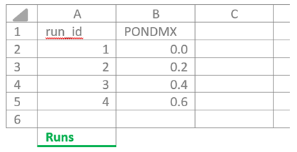
Once all variables in the SWAP-template(s) have been selected, Excel can be used to define their values. There are a few restrictions to follow. The Excel file must include a worksheet names Runs containing a column run_id, which should be a sequence from 1 to \(n\). Each run_id represents a single SWAP simulation. Variable values can be linked directly to the run_id, as illustrated for PONDMX below.
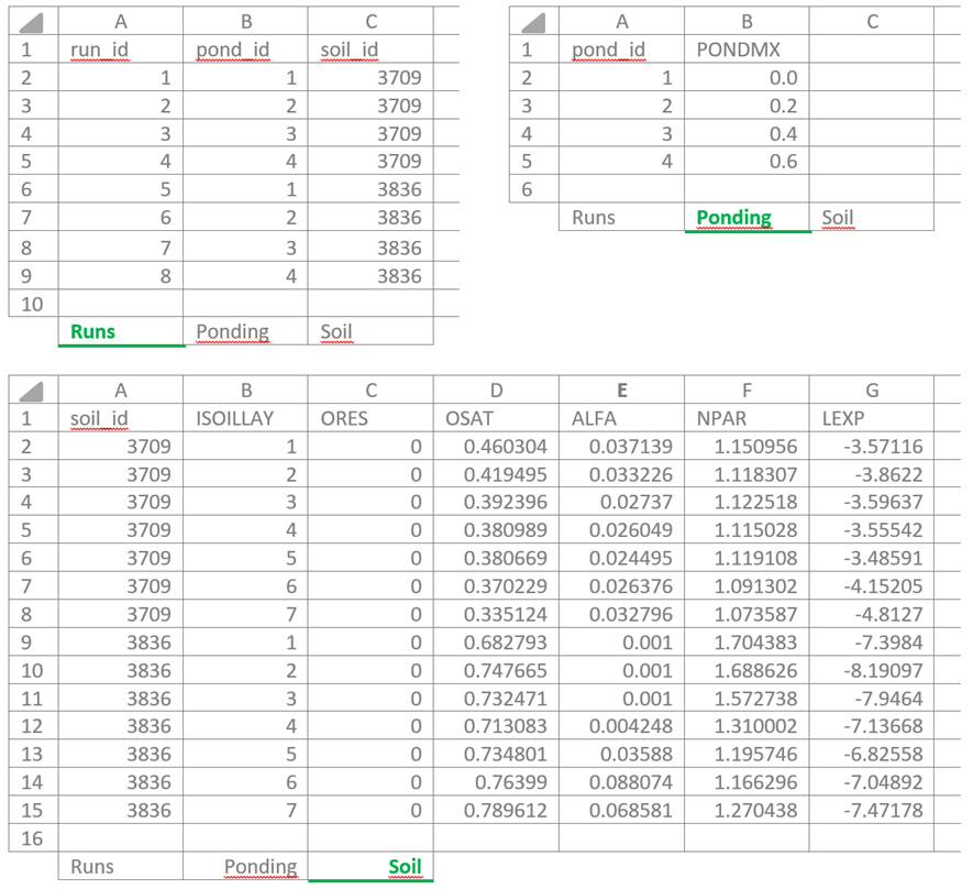
Another way to associate variables with a specific run_id is by using a so-called key. This key may consist of a single column or a combination of columns, all of which must have names ending in *._id. In a separate worksheet, variable values can then be linked to the run_id via this single- or multi-column key.
Variables that depend on an index such as date (DATE), depth or soil layer (ISOILLAY), or development stage (DVS) can be defined using a key together with an additional index column. In the example below, the maximum ponding depth is varied for two soil types using three worksheets (Runs, Ponding, and Soil), resulting in a total of eight SWAP simulations.
In case of a so-called switch variables it is allowed to leave cells empty, see example below.
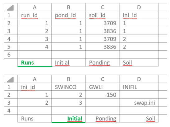
In Excel, the use of formulas is allowed. Comments can be added by labeling the top row with “#”.
1.3 Execute SWAP simulations
Once the SWAP templates and the corresponding Excel file are prepared, the simulations can be executed. This is done using a single R script, run_swap.R. The script requires a plain text file, a so-called control file (in this case control.inp):
The control file is used to define various options and to specify paths to input files and directories. The user is responsible for organizing the data in a logical structure (the control file supports relative paths such as ‘./’ and ‘../’). Paths and options are identified using specific keywords that must not be modified. Comments can be included in the control file by using ‘#’.
The R-script run_swap.R consist of three separate procedures: a pre-process, a main-process and a post-process, which can be executed independently (see example below). The pre-process creates a SQLite database based on the information in the Excel file; using SQLite enables parallel execution through multicore processing. The main process then runs all or a selected subset of SWAP simulations.
Optionally, a post-process can be used to analyse the model results. This is discussed in Chapter 2.