1 Model overview
1.1 Model domain and processes
SWAP simulates transport of water, solutes and heat in the vadose zone in interaction with vegetation development. The model employs the Richards equation including root water extraction to simulate soil moisture movement in variably saturated soils. In addition to ordinary matrix flow, SWAP considers flow through macropores as may occur in clay and peat soils. Solute transport includes the basic processes convection, dispersion, adsorption and decomposition. For more detailed solute transport studies, SWAP can be used in combination with specialized chemical transport models such as PEARL for pesticides and Soil-N or ANIMO for nitrogen. SWAP simulates soil heat flow taking into account actual heat capacities and thermal conductivities. The generic crop growth module WOFOST is incorporated to simulate leaf photosynthesis and plant growth. The soil moisture, heat and solute modules exchange status information each time step to account for their interactions. On a daily basis crop growth is affected by actual conditions of weather, soil moisture and salinity. An extensive test protocol ensures the numerical code quality of SWAP.
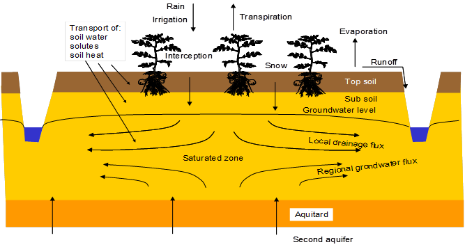
In the vertical direction the model domain reaches from a plane just above the canopy to a plane in the shallow groundwater (Figure 1.1). In this zone the transport processes are predominantly vertical, therefore SWAP is a one-dimensional, vertical directed model. The flow below the groundwater level may include lateral drainage fluxes, provided that these fluxes can be prescribed with analytical drainage formulas. The model is very flexible with respect to input data at the top and bottom of the soil column. At the top in general daily weather conditions will suffice. For Nordic conditions a simple snow storage module has been implemented. In case of more focussed studies (e.g. runoff or diurnal transpiration fluxes) evapotranspiration and rainfall data can be specified in more detail. At the bottom various forms of head and flux based conditions are used.
In the horizontal direction, SWAP’s main focus is the field scale. At this scale most transport processes can be described in a deterministic way, as a field generally can be represented by one microclimate, one vegetation type, one soil type, and one drainage condition. Also many cultivation practices occur at field scale, which means that many management options apply to this scale. Upscaling from field to regional scale for broader management policy studies is possible with geographical information systems.
The smallest time steps in SWAP are in the order of seconds for fast transport processes such as intensive rain showers with runoff or flow in macroporous clay soils. These time steps are automatically increased in periods with more slow flow conditions. Depending on simulation complexity, computation times for 50 year periods range from 30 to 500 seconds on ordinary personal computers.
1.2 SWAP installation
SWAP installation.
The SWAP model can be downloaded from Internet site swap.wur.nl. This site contains general information on model features, applications and test reports. Various SWAP versions are available at the Internet site. This manual applies to SWAP 4.3. Only the most recent SWAP version is supported by the SWAP team.
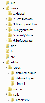
To allow installation on different operating system, we compiled a versatile set for distribution and packed all files into one zip-file. The zip-file can be unpacked on an arbitrary folder. Once unpacked a number of subfolders are created (Figure 1.2), which contain:
- Swap executable
- Swap source code
- User manual
- Several case studies
- Additional input data:
- Daily weather data of Wageningen meteorological station of the period 1971-2000.
- Simple crop input data for grass, fodder maize, potato, sugar beet and winter wheat.
- Detailed crop input data for winter wheat, grain maize, spring barley, rice, sugar beet, potato, field bean, soy bean, winter oilseed rape and sunflower.
SWAP can be automatically launched for the example Hupsel. Also runs can be made with the other 5 case studies described in Chapter 12.
1.3 Model input
The input data of SWAP are divided over 4 different file types:
- Main input file (*.swp)
- Meteorological file (*.met, *.rain or *.yyy)
- Crop growth file (*.crp)
- Drainage file (*.dra)
Tip 1.1 provides an overview of the information in these input files. The main input file and the meteorological data file are always required. Input files of crop growth and drainage are optional. The extensions of the files are fixed, with the exception of meteorological (and rainfall) data supplied in annual files, for which the extension equals the last three digits of the year (e.g. 2017 yields .017). The names of the input files are free to choose and are specified in the main input file. As listed in Tip 1.1, the main input file contains general information with regard to the simulation, meteorology, crop rotation scheme, irrigation, soil water flow, heat flow and solute transport. For meteorological data, commonly a file with daily data is used. In Chapter 3 also more detailed input of evapotranspiration and rainfall fluxes will be discussed. The detailed crop growth input file is required to simulate crop development and biomass assimilation. As an alternative, the development of crop parameters as leaf area index or rooting depth can be prescribed in the simple crop growth input file. The drainage input file contains two sections. The first, basic drainage section provides input for drainage towards ditches and/or drains. The second, extended drainage section provides input for drainage including simulation of surface water levels.
SWAP uses the TTUTIL library (Van Kraalingen and Rappoldt 2000) for reading input files. Tip 1.2 gives an example of a part of the *.swp input file. General rules for the format of input files are:
- free format with the structure ‘VARIABLE_NAME’ = ‘value’ or, in case of arrays, in a table with variable names in the first line;
- order of variables is free;
- comment in lines is allowed starting with symbols ‘*’ or ‘!’;
- blank lines are allowed.
The input files list of each parameter their symbolic name, a description and an identification. The identification between square brackets provides information on:
- the range
- the unit
- the data type (I = integer, R = real, Ax = character string of length x) For example: [-5000 .. 100 cm, R] means: value between -5000 and +100 with a unit in cm, given as a Real data type (which means that the value in the input file should contain a dot).
SWAP will read times according to the following format: 2017-02-10_16:30:00.00 denotes February 10, 2017 at 4.30 PM. If in the input only dates and no times are specified, SWAP will assume time 0:00. In case of input data series as function of time (e.g. groundwater levels) or depth (e.g. initial pressure heads), SWAP will apply linear interpolation for times and depths in between. Outside the specified range, the closest value will be adopted. For instance in Tip 1.2, the rainfall intensity (raintb) will gradually increase from 20 to 40 mm d-1 between t = 1.0 and t = 360.0 d. At t > 360.0 d, the rainfall intensity will be 40 mm d-1.
1.4 Model run
The most common way to run SWAP is by executing a batch file, which refers to the SWAP executable and the main input file *.swp. The batch file and the *.swp file need to be present in the same directory. The *.swp file contains the names and locations of other input files. In this way the meteorological, crop and drainage data can be specified on separate folders.
An example of the batch file is given in Tip 1.3. In this case SWAP will use hupsel.swp as main input file. If no name is specified behind the executable call, SWAP assumes swap.swp as main input file. The pause statement keeps the window box with screen messages open; this is convenient when runtime warnings or errors occur.
An alternative to run SWAP is by double-clicking file swap.exe. In that case the main input file should be called swap.swp, and should be located in the same folder as file swap.exe.
Three types of messages may occur during a model run:
- error messages with respect to the input data
- warnings with the advise to adapt the combination of selected options because the specified combination is not feasible
- fatal calculation errors which stop the simulation
Output files are created in the same directory as the main input file. The log file, named *.log, contains details on the iteration statistics. If the simulation completes successfully, the file ends with the message: ‘SWAP simulation okay!’. Any warnings generated during the simulation are stored in the file *wrn. If an error occurs, the simulation stops, and the corresponding error message is recorded in the file *.err.
1.5 Model output
Output from SWAP is stored in general ASCII files, which can be read with any editor or word processor. Some output files are always generated, other files are optional. Tip 1.4 provides an overview of the variables that are printed in each output file. All output files have the common header containing the project name, file description, file name, model version and the time of generation. SWAP allows users to define a custom set of output variables and store them in a single file (*_output.csv), which can be easily imported into Excel (see Appendix A for further details). The output interval may range from 0.001 day to 1.0 year. If the output time only consists of a date, the output represents the situation at the end of the particular day. We may distinguish output of state variables and incremental fluxes since the last output time. The output file with final values of state variables (*.end) can be used as input for a subsequent simulation period. This might be useful to derive suitable initial conditions.
In addition to the ASCII files, formatted and unformatted (binary) export files can be generated with data that cover the entire simulation period. These output files can be used as input for advanced solute transport models, such as PEARL (Leistra et al. 2001) for pesticides and ANIMO (Groenendijk, Renaud, and Roelsma 2005) for nutrients. A description of these export files is given in Appendix B.
1.6 Case studies
Chapter 12 contains 4 case studies with SWAP. The input files of these cases come with the installation of SWAP. The case studies are:
- Hupsel Brook
- Grass growth
- Macropore flow
- Salinity stress
The first case of a field in Hupsel Brook catchment includes a simulation with 3 different crop growth modules. This case is used to illustrate the input files in this SWAP manual.
1.7 Reading guide
In the next chapters we discuss subsequently:
- Soil water flow (Chapter 2)
- Evapotranspiration and rainfall interception (Chapter 3)
- Surface runoff, interflow and drainage (Chapter 4)
- Surface water system (Chapter 5)
- Macropore flow (Chapter 6)
- Crop growth (Chapter 7)
- Solute transport (Chapter 8)
- Soil heat flow (Chapter 9)
- Snow and frost (Chapter 10)
- Irrigation (Chapter 11)
- Case studies (Chapter 12)
- Verification and validation (Chapter 13)
- Sensitivity analyses (Chapter 14)
- Calibration (Chapter 15)
The first part of Chapter 2 describe the physical relations incorporated in SWAP. This part also describes implemented numerical procedures, if required to use SWAP in a proper way. The second part of each chapter describes the model input. If relevant, suggestions for input are included.
The appendices contain information on:
- User defined output (Appendix A)
- Formatted and unformatted binary output files (Appendix B)
- Equations for the implicit linearization of hydraulic conductivities (Appendix C)
- Equations for the partial derivatives of Fi to pressure heads (Appendix D)
- Numerical scheme of soil water boundary conditions (Appendix E)
- Application of the Penman Monteith method (Appendix F)
- Tables with critical pressure heads for root water extraction (Appendix G)
- Solution procedure process-based root water uptake models (Appendix H)
- Derivation and examples of macropore equations (Appendix I)
- Shrinkage characteristic data (Appendix I)
- Tables with salt tolerance data (Appendix J)
- Equations for the numerical solution of heat flow (Appendix L)
1.8 Area of application
The core of SWAP is formed by the general water movement equation in porous media (soil). This is a non-linear, partial differential equation. It has to be solved by numerical mathematics, and the solution is determined by the initial and boundary conditions of the system considered. Technically the implementation of the numerical solution procedure in SWAP has been verified via comparison with analytical solutions (see Chapter 13): from the good correspondence it can be concluded that the core of SWAP is well programmed. Applications of SWAP in practice are fully determined by the user-supplied initial condition and boundary conditions. This is part of the modelling that depends on the user, for which SWAP offers several options and sub-models. The result of the SWAP simulation is highly dependent on the user-supplied information (remember: garbage in = garbage out).
SWAP is primarily meant for simulating one-dimensional situations (vertical water movement), with possibilities of exchange of water with the surroundings via drainage and/or infiltration to/from drainage systems (drain tubes, ditches, canals); SWAP can thus be seen as quasi-three-dimensional. SWAP results should be seen as outcome for the square-meter scale up to the scale of a single field or parcel. For larger areas several SWAP runs need to be performed. Horizontal exchange of water between individual SWAP soil columns is not automatically possible.
For detailed 2D or 3D calculation SWAP cannot be used; for example, the determination of the extent of the wetted bulb underneath a dripper cannot be simulated.
1.9 Major assumptions in SWAP
SWAP is based on the following major assumptions:
- water movement is dominantly one-dimensional (vertical); quasi-three-dimensional aspect have been included as exchange with drainage systems (drain tubes, ditches, canals; infiltration from these systems into the soil can also be considered);
- water movement in porous media requires that the porous medium (soil) is rigid, isotropic, isothermal and water is incompressible; swelling and shrinking can be partly considered in case the option macropore flow is used;
- only single phase flow (water) is considered; air in the soil always remains at atmospheric pressure;
- soils can be variably saturated;
- soils can be heterogeneous: the soil then consists of different soil layers each with its own soil physical properties; in principal these are given by the Mualem – van Genuchten equations (other relationships could be provided as tabulated input data); hysteresis can be considered when the Mualem-van Genuchten relationships are used;
- top and bottom boundary conditions can be either flux-controlled or pressure head controlled; at the bottom boundary several options can be considered; at the top a pressure head condition cannot be supplied by user but only occurs internally when ponding arises;
- transpiration reduction can be caused due to drought, lack of oxygen (too wet) or too saline conditions; transpiration reduction is used in WOFOST to predict crop growth reduction;
- ponding at the soil surface occurs when the infiltration capacity is exceed; surface runoff occurs after a threshold ponding height is exceeded and is calculated in analogy to Manning’s overland flow;
- multiple level drainage systems can be considered to mimic discharge in a sub-catchment; imposed water levels in these drainage systems can be considered;
- macropore flow can be considered as a special case (e.g. for structured soils such as clay and peat); shrinkage and swelling of these macropores can be included;
- the crop is explicitly simulated in SWAP via incorporation of the WOFOST model for major arable crops (maize, potato, sugar beet, winter wheat, (summer) barley); for grassland a detailed crop growth module was derived according to the same philosophy as WOFOST; other crops can be simulated via a simple crop growth module;
- solute transport is described by the dispersion-diffusion – convection equation including simple transformation equations, adsorption and root uptake; for more detailed solute transport coupling of SWAP with ANIMO (Groenendijk et al. (2005); Renaud et al. (2005) is suggested; a simple single-layer N-module is present (Groenendijk et al. (2016));
- soil temperature can be simulated as a diffusion process; soil temperatures can influence crop growth, solute transformations etc.;
- simple snow and frost options are available (requires soil temperature);
- irrigation can be considered either as fixed times and quantities, or chosen from five trigger options and three irrigation depth (amount) criteria.
1.10 Summary of fitness-for-use
SWAP can be downloaded from the website (swap.wur.nl) and comes as a zip-file. This file can be unzipped to any folder. No formal installation procedure is required (no administration right is needed). Standard, SWAP is available as an executable for Windows platforms. The source code is available, so that users are able to produce their own executables e.g. for Linux platforms; from own tests we know that SWAP can be compiled and run under Linux without changes in the source code.
SWAP is not a simple, graphically oriented plug-and-play application. The user must supply information in ASCII input files and then run SWAP by hand indicating the name of the main input file (*.swp); see general description Section 1.4. After completion of the model run, the results are available in several output ASCII files. The user can use these in their own scripts for further analyses.
Basically, based on meteorological information, crop parameters, soil properties, initial and boundary conditions SWAP predicts as a function of time the different water balance components in this system. It is the user that supplies all the necessary information, which will be used by the in SWAP implemented theories to predict the fate of water. Output is available as a function of time which can be further analysed by the user.
SWAP is also used in Wageningen University courses. For this a specific graphical user interface was developed so that students can easily change major input information and visualize major output information. Since not all functionalities of SWAP have been incorporated in this GUI, this interface is not distributed together with SWAP download.
1.11 Brief critical analysis of possible shortcomings
The SWAP model is basically a calculator that solves a partial differential equation based upon input information (initial and boundary conditions) as supplied by the user. Technically, the core of the model has been verified against analytical solutions (see Chapter 13). This means that the quality of the output for a user-defined situation is then mainly determined by the quality of the input as supplied by the user (garbage in = garbage out). This is something that cannot be controlled or checked by the model code. The only check performed by the model is done by checking the input values against pre-defined ranges in the source code.
SWAP is basically a point-model in space and only considers depth along which variable soil conditions can be considered. Real soils are heterogeneous, soil water movement may sometimes be 2- or 3-dimensional (e.g., underneath drip irrigation), and soils and their properties may change in time (e.g., swelling-shrinking; compaction). These aspects cannot be considered in a single SWAP run.
See further the description provided on major assumption (Section 1.9) and fitness-for-use (Section 1.10).
1.12 Brief global uncertainty analysis
As mentioned above, SWAP is basically a simulation model for one-dimensional problems (a point model in terms of surface area). By adding the possibilities of side boundary conditions mimicking possible exchange with the surrounding via different levels of drainage/infiltration boundaries, the SWAP application can thus be extended to a field or parcel. However, the outcome still refers to a vertical distribution of state variables. As such, it cannot predict horizontal variation within the field. Comparison with measured field data (e.g., groundwater level, water content, crop yield) can show a mismatch since, for example, the groundwater level gauge may have been installed at a position that is not comparable with the (average) information that was used as input in the model. This means that uncertainty in model outcome is likely present.
Below a brief and global description regarding uncertainty is provided. Such an analysis should focus on the following aspects: context, model, inputs, parameters, output (Walker et al. 2003; Janssen et al. 2003).
Context
SWAP is used on a diversity of projects and research questions with focus on the water balance in the unsaturated-saturated top part (down to one to a few meters) of soils, often in relation to agricultural crop production. Often, these involve studies where geographic differences need to be studied. For that relevant information needed as input should be available at the scale of interest. In order to simulate a region this means that several stand-alone SWAP simulations are needed which are representative for a small area of the total region of interest. The geographical variability in the outcome is then purely driven by the input information. SWAP is a pure technical model and does not include economics, social and political aspects.
Model
Technically, the numerical solution for water movement, solute transport and soil temperature has been verified against analytical solutions, and validation against field data has been performed (see Chapter 13). This, however, does not guarantee certainty in overall SWAP model outcome.
Over the decades the structure of the model has evolved and likely there is a good logistics in exchange of information between the different modules and the sequence in which these modules are used. Several modules are present in SWAP but not all are as sophisticated as others.
In scientific community different descriptions exist for different processes, indicating that there is no universal description available. In SWAP some processes have different alternatives that can be used, either i) depending on data availability or ii) on desired details for which a subprocess needs to be considered. As an example for i): for crop growth it is advised to use the WOFOST module for those types of crops for which default WOFOST data files are available; when other crops need to be considered SWAP offers a simplified crop growth module. As an example for ii): root water uptake is often modelled via the so-called Feddes reduction model in SWAP, but alternative root water uptake models are available that take into account the root-soil interface. One such detailed root water uptake model is already implemented in SWAP and another one will be implemented soon.
There is an option to include snow and frost in SWAP. This is done in a simple way, as these processes hardly play a role for (current) Dutch conditions. A detailed macropore option is present in SWAP. It is not used often, since it requires many input parameters for which data are lacking. Soil temperature can be simulated, and is required in case solute transport or the N-module is considered. Soil temperature is dependent on soil volumetric water content, but heat transport via moving water is not included.
Inputs
The outcome of a SWAP simulation is highly driven by the quality of the input information. In the Netherlands, modellers (users) likely will make use of information obtained from the Dutch soil map, the Staring series (Heinen, Bakker, and Wösten 2020) or the derived soil physical units map BOFEK2020, which is derived from the soil map and the Staring series (Heinen et al. 2021). Some crop parameters can be obtained from the standard WOFOST database, but for other crops this information must be obtained via expert judgement.
Parameters
In SWAP most of the information needed to perform the simulation is based on information provided by the user (via text input files). In some cases universal or literature constants (parameters) have been hard coded (mostly as parameters in the top of the routine/function/module). For official releases the source code is available and then these parameters might be changed if needed. In the future we might consider to have all hard coded parameters listed in a special parameter input file. This, however, only provides more flexibility, and will not automatically lead to more certain outcome.
Model outcomes
Many outcome variables are available, and users are able to indicate what information they want as output. The output itself comes as is, i.e., no qualitative or quantitative information on the reliability or uncertainty of the outcome is given.
All-in-all, SWAP-WOFOST fulfills the need of having a simulation tool that can consider the water balance in the combined soil-crop domain. It makes use of universally accepted process descriptions, and it is widely used both nationally and internationally, indicating that it is an accepted tool for this type of research problems. Despite this acceptance as well as some shortcomings in the model, we are aware that the modelling outcome comes with uncertainties. Such shortcomings are less likely the result of errors in the numerical implementation (solution) of the governing differential equations, and are more due to uncertainties in the available input information. Therefore, it is strongly advised that for each new study (application) the user should perform some kind of sensitivity analysis to determine where possible problems or uncertainties in outcome may arise.