Appendix I — Derivation of some macropore geometry equations
Basis of the determination of the effective vertical macropore wall area and the effective crack width is the assumption that the natural variety of soil matrix polygons can be described in terms of one effective regular soil matrix polygon. Crucial condition for this polygon is that many of it should fit together without any gaps to ‘tile the plane’. From the regular polygons, only equilateral triangles, squares and regular hexagons have this quality. Empirical experience points out that squares and hexagons in particular are the most likely candidates for these polygons. Which of the two should be chosen, is irrelevant. They are both regular polygons with an even number of sides. All of these even-sided regular polygons, from square to circle, have two relevant, special qualities: the quotient of their perimeter divided by their area is independent of the number of sides and their area is a function of the squared diameter.
Effective vertical macropore wall area
All even-sided regular polygons with \(n\) sides are built up of \(n\) equal isosceles triangles with base of length \(x\) (cm) and height 0.5 \(d_{pol}\) (cm) (Figure I.1). The perimeter of the polygon equals \(n\) times \(x\) and the area equals \(n\) times the area of the triangle. The latter equals 0.25\(d_{pol}\) \(x\) (cm2), so that:
\[ \frac{perimeter_{pol}} {area_{pol}} = \frac{nx} {n0.25d_{pol}x} = \frac{4} {d_{pol}} \tag{I.1}\]
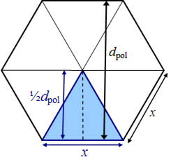
The vertical area of the wall of the polygon of Figure I.1 per unit of depth is equal to the perymeter of the polygon. In order to express this area per unit of horizontal area it is divided by the area of the polygon. Thus, the effective vertical area of the wall of the matrix polygons \(A wall\) per unit of depth and horizontal area, which implies per unit of volume, equals the quotient of the polygons’ perimeter divided by their area, which equals \(\frac{4}{d_{pol}}\) (cm-1).
Effective crack width
For even-sided regular polygons it can be derived that their sides \(x\) (Figure I.1) can be expressed as \(\frac{C_n}{n}d_{pol}\), where \(C_n\) (-) is a constant that depends on \(n\). For squares, hexagons and circles, \(C_n\) equals, \(4\), \(2\sqrt{3}\) and \(π\), respectively. With \(C_n\) a general equation for the area \(A_{pol}\) (cm2) of an even-sided regular polygon as function of \(d^2_{pol}\) can be derived:
\[ A_{pol} = 0.25nd_{pol}x = 0.25nd_{pol}\frac{C_n}{n}d_{pol} = 0.25C_n d^2_{pol} \tag{I.2}\]
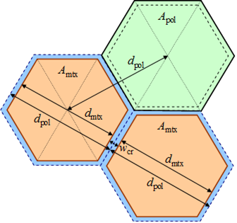
For this equation, we define \(d_pol\) as the distance between the centres of two adjacent basis polygons (Figure I.2). The value of this diameter is fixed. The value of the actual soil matrix polygon diameter \(d_{mtx}\) depends on the crack width, which is not fixed in case of a shrinking matrix. Thus, the crack width wcr can be calculated as (Figure I.2):
\[ w_{cr} = d_{pol} - d_{mtx} \tag{I.3}\]
The horizontal area of the cracks \(A_{cr}\) (cm2) as fraction of \(A_{pol}\) depends on the macropore volume fraction \(V_{mp}\) (cm3 cm-3) as:
\[ A_{cr} = V_{mp} A_{pol} \tag{I.4}\]
The horizontal area of the matrix polygon \(A_{mtx}\) (cm2) is a function of \(d^2_{mtx}\) according to Equation I.2:
\[ A_{mtx} = 0.25C_n d^2_{mtx} \tag{I.5}\]
\(A_{mtx}\) is also equal to the difference between basis polygon area \(A_{pol}\) and crack area \(A_{cr}\):
\[ A_{mtx} = A_{pol} - A_{cr} = A_{pol} - V_{mp}A_{pol} = \left(1-V_{mp}\right)A_{pol} = \left(1-V_{mp}\right)0.25C_n d^2_{pol} \tag{I.6}\]
Combining the right hands terms of Equation I.5 and Equation I.6 yields:
\[ 0.25C_n d^2_{mtx}= \left(1-V_{mp}\right)0.25C_n d^2_{pol} \tag{I.7}\]
and:
\[ d^2_{mtx} = \left(1-V_{mp}\right)d^2_{pol} \tag{I.8}\]
so that:
\[ d_{mtx} = d_{pol}\sqrt{1-V_{mp}} \tag{I.9}\]
And finally, the crack width is expressed as:
\[ w_{cr} = d_{pol} - d_{mtx} = d_{pol} \left(1 - \sqrt{1-V_{mp}}\right) \tag{I.10}\]
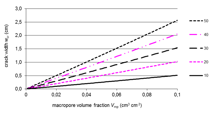
Figure I.3 shows the crack width \(w_{cr}\) as function of the macropore volume fraction \(V_{mp}\) for different polygon diameters \(d_{pol}\).
Effect of crack width \(w_{cr}\) on calculation of area of vertical wall \(A^*_{wall}\) and distance \(x_{pol}\)
Strictly speaking, the vertical macropore wall area \(A^*_{wall}\) and the horizontal distance \(x_{pol}\) should be calculated on the basis of \(d_{mtx}\) instead of \(d_{pol}\). However, \(x_{pol}\) is used in combination with \(A^*_{wall}\) as: \(\frac{A^*_{wall}}{x_{pol}}\) (Equation 6.49 and Equation 6.53). This quotient is similar for using \(d_{mtx}\) and \(d_{pol}\):
\[ \frac{A^*_{wall,mtx}}{x_{pol,mtx}} = \frac{\frac{4}{d_{mtx}}\frac{A_{mtx}}{A_{pol}}}{0.5d_{mtx}} = \frac{\frac{4}{d_{mtx}} \frac{d^2_{mtx}}{d^2_{pol}}} {0.5d_{mtx}} = \frac{4}{0.5d^2_{pol}} = \frac{A^*_{wall}}{x_{pol}} \tag{I.11}\]
Only in Equation 6.42, the calculation of the absorption, \(A^*_{wall}\) is used without dividing by \(x_{pol}\). In that case, \(A^*_{wall,mtx}\) is used for \(A^*_{wall}\). Therefore, \(A^*_{wall}\) is corrected with Equation I.9 according to:
\[ A^*_{wall,mtx} = \frac{d_{mtx}}{d_{pol}} = \frac{d_{pol}\sqrt{1-V_{mp}}}{d_{pol}} A^*_{wall} = \sqrt{1-V_{mp}} A^*_{wall} \tag{I.12}\]
Examples of macropore geometry realizations
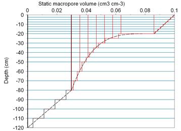
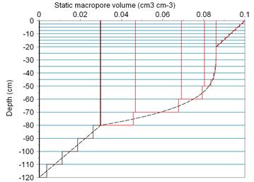
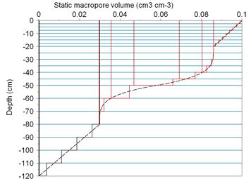
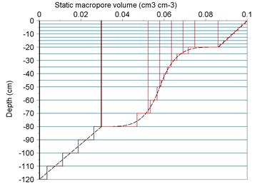
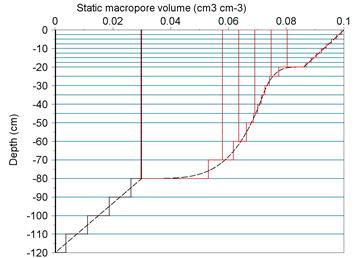
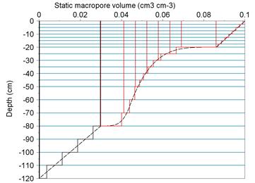
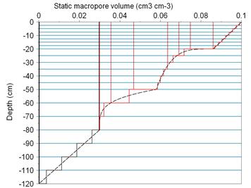
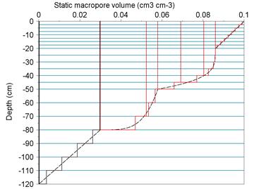
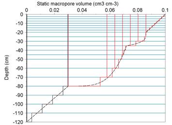
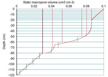
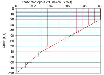
The basic setup of the macropore geometry cases is described in Section 6.2.1. In the examples below, the red vertical lines indicate the IC sub-domains, with domains ending in the same compartment (horizontal blue lines) lumped together. A basic example is given in Figure I.4. The Figures thereafter build upon the first Figure, with altered parameters described in their captions.
\[ \begin{align} \\ VLMPSTSS & = V_{st,0}\\ PPICSS & = P_{ic,0}\\ NUMSBDM & = n_{sd}\\ POWM & = m\\ RZAH & = R_{ZAh}\\ SPOINT & = S_p\\ SWPOWM & = Sw_{powm}\\ \end{align} \]