| Soil | \(\theta_r\) (cm3 cm-3) | \(\theta_s\) (cm3 cm-3) | \(\alpha\) (cm-1) | \(n\) (-) | \(\lambda\) (-) | \(K_s\) (cm d-1) |
|---|---|---|---|---|---|---|
| Clay | 0.100 | 0.40 | 0.01 | 1.1 | 0.5 | 10 |
| Loam | 0.080 | 0.43 | 0.04 | 1.6 | 0.5 | 50 |
| Sand | 0.045 | 0.43 | 0.15 | 3.0 | 0.5 | 1000 |
14 Sensitivity analyses
14.1 Introduction
Numerical simulation models are by definition approximations of reality. The outcome of model predictions highly depends on the boundary conditions, initial condition, model parameters, and on the numerical discretization (both in space and in time). The processes considered in SWAP, i.c. water movement and solute transport, are highly non-linear. Therefore, finding out the sensitivity of the model with respect to its model input cannot be determined analytically. Especially not for time-dependent, dynamic situations. For specifically defined situations analytical solutions for steady-state situations are sometimes available. Since the number of input variables and choices in sub-processes in SWAP is rather large, there is no unique simple sensitivity procedure available, nor has it been carried out in detail. It is suggested that for each study the modeller performs a problem-unique sensitivity analysis to determine which input variables need to be determined in detail. This chapter will provide the following sensitivity analyses:
- the effect of spatial and temporal discretization of the SWAP model based on two analytical, steady-state situations for water movement (Section 4.2) and solute transport (Section 14.3);
- the effect of spatial and temporal discretization for an infiltration-runoff situation supplemented by analytical expressions of the sensitivity of the runoff equation (Section 14.4);
- the effect of spatial discretization upon a capillary rise situation (Section 14.5);
- a Monte-Carlo type sensitivity analysis for a set of input parameters from the Watervision Agriculture project (Section 14.6);
- brief descriptions of sensitivity analyses using SWAP performed in scientific literature (Section 14.7).
14.2 Steady-state water movement
This example is based on one of the default test cases to which each new release of SWAP is tested. It refers to a steady-state infiltration problem in a soil column consisting of two contrasting soil layers. The problem is fully described in Vanderborght et al. (2005). The steady-state solution is given by:
\[ \Delta z = {z_1} - {z_2} = - \int\limits_{h\left( {{z_2}} \right)}^{h\left( {{z_1}} \right)} {\frac{{K\left( h \right)}}{{I - K\left( h \right)}}{\rm{d}}h} \tag{14.1}\]
where \(z\) is the soil depth (cm), \(h\) is the pressure head (cm), \(K\) is the hydraulic conductivity (cm d-1), and \(I\) is the infiltration rate (cm d-1). No analytical solution is available to solve Equation 14.1, so that it is numerically approximated by increasing \(z\) starting at the bottom of the soil profile with small steps in \(\Delta z\) (e.g., 2-13 cm) until soil surface is reached, and where the hydraulic properties change at the interface of the soil layers. The pressure head at the bottom (total soil depth 200 cm) was obtained from the hydraulic conductivity relationship such that \(K(h)\) = \(I\) (unit gradient bottom boundary condition). For each new depth \(z\) the corresponding \(h\) follows then from
\[ h\left( z \right) = h\left( {z - {\rm{d}}z} \right) - {\rm{d}}z\left( {\frac{I}{{K\left( {h\left( {z - {\rm{d}}z} \right)} \right)}} + 1} \right) \tag{14.2}\]
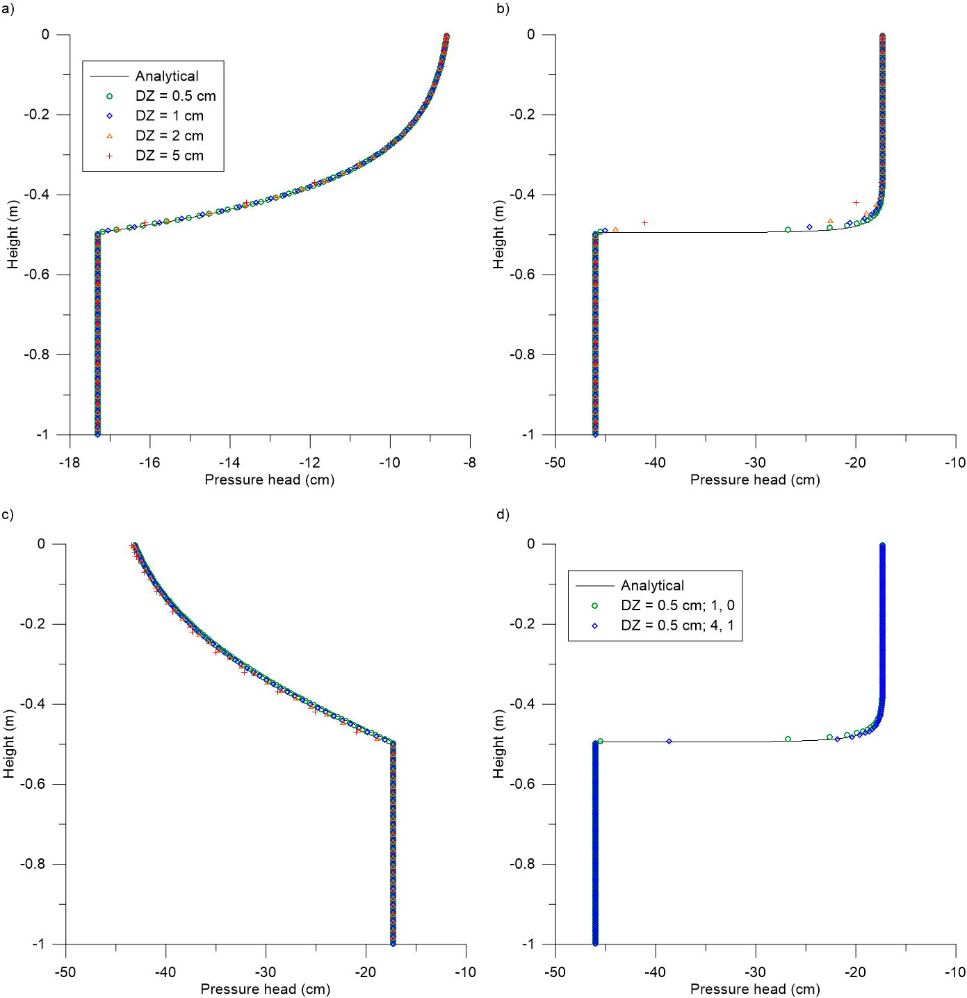
Three situations were considered: 49.5 cm clay on sand and 49.5 cm sand on loam and 49.5 cm loam on sand. The constant infiltration rate was \(I\) = 0.5 cm d-1 and the Mualem-van Genuchten parameters for the soils are listed in Table 14.1. Note: In Vanderborght et al. (2005) the first layer was 50 cm thick; here 49.5 cm is used corresponding to the first test case of SWAP, where it was chosen to have the first layer equal to 0.5 cm (see later) followed by layers of 1 cm resulting in the default test case having the first soil layer being 49.5 cm. Note that erroneously in the first test case of SWAP the SWAP results are compared to the analytical solution with first soil layer equal to 50 cm (instead of 49.5 cm).
The infiltration started at \(t\) = 0, and the simulated steady-state profiles were obtained at \(t\) = 365 d. Simulation were performed for the following spatial discretizations of the soil profile: \(\Delta z\) = 0.5 cm, 1.0 cm, 2.0 cm and 5.0 cm. In all cases the first layer was always 0.5 cm thick; therefore, for the third discretization the second layer was set equal to 1 cm, and for the fourth discretization the layers 2-5 were set equal to 1 cm (Table 14.2).
| Case | Description |
|---|---|
| \(\Delta z\) = 0.5 cm | \(\Delta z\) = 0.5, 98x0.5, 300x0.5 cm |
| \(\Delta z\) = 1.0 cm | \(\Delta z\) = 0.5, 49x1.0, 150x1.0 cm |
| \(\Delta z\) = 2.0 cm | \(\Delta z\) = 0.5, 1.0, 24x2.0, 75x2.0 cm |
| \(\Delta z\) = 5.0 cm | \(\Delta z\) = 0.5, 4x1.0, 9x5.0, 30x5.0 cm |
Figure 12 presents the comparison between the simulated and analytical solutions for both cases (some statistics in Table 3). For the cases clay-on-sand and loam-on-sand the pressure head profiles in the clay and loam top soils moderately change towards the layer interface, and we do not see big differences between the spatial discretizations employed. For the sand-on-loam case there is a sharp infiltration front near the layer interface. For this case a big effect of the chosen discretization is seen, where the coarser discretizations differ markedly from the analytical solution.
For the case sand-on-loam an additional simulation was performed with thin layers (\(\Delta z\) = 0.5 cm) for which in the numerical solution of SWAP the unknown hydraulic conductivity \(K\) is taken implicitly into account during the iterative solution (swkimpl = 1 (default 0)) and where the hydraulic conductivity at the interfaces of the grid layers is calculated as the geometric average of the two neighbouring nodes (swkmean = 4 (default 0)). An improvement can be seen in the performance (Figure 12.1 d; new case denoted as \(\Delta z\) = 0.5 cm; 4, 1).
These examples show that spatial discretization can be important for situation where one expects great gradients in the soil profile.
| Case | Description | \(r^2\) | RMSE | NRMSE |
|---|---|---|---|---|
| Clay on sand | \(\Delta z\) = 0.5 cm | 0.9999942 | 0.0083752 | -0.0005351 |
| \(\Delta z\) = 1 cm | 0.9999765 | 0.0169193 | -0.0010822 | |
| \(\Delta z\) = 2 cm | 0.9999047 | 0.0343902 | -0.0022096 | |
| \(\Delta z\) = 5 cm | 0.9994891 | 0.0871275 | -0.0058113 | |
| Sand on loam | \(\Delta z\) = 0.5 cm | 0.9934949 | 0.9944481 | -0.0255111 |
| \(\Delta z\) = 1 cm | 0.9843302 | 1.5505950 | -0.0398373 | |
| \(\Delta z\) = 2 cm | 0.9655142 | 2.3952998 | -0.0629153 | |
| \(\Delta z\) = 5 cm | 0.9382829 | 3.3572274 | -0.0908891 | |
| \(\Delta z\) = 0.5 cm; 4, 1 | 0.9975062 | 0.6145829 | -0.0157662 | |
| Loam on sand | \(\Delta z\) = 0.5 cm | 0.9999733 | 0.0566082 | -0.0026558 |
| \(\Delta z\) = 1 cm | 0.9998984 | 0.1117148 | -0.0052278 | |
| \(\Delta z\) = 2 cm | 0.9996393 | 0.2171401 | -0.0100602 | |
| \(\Delta z\) = 5 cm | 0.9986929 | 0.4903657 | -0.0210330 |
14.3 Steady-state solute transport
This example is based on one of the default test cases to which each new release of SWAP is tested. For a soil column with uniform downward water movement and where a pulse of a solute is applied at the soil surface, the concentration inside the soil column can be analytically described as a function of time and depth (J. G. Kroes and Rijtema 1996; based on Jury and Roth 1990):
\[ c = \frac{M}{{\theta R}}\exp \left[ { - kt} \right]\left( {\frac{1}{{\sqrt {\pi D\frac{t}{R}} }}\exp \left[ { - \frac{{{{\left( {z - v\frac{t}{R}} \right)}^2}}}{{4D\frac{t}{R}}}} \right] - \frac{v}{{2D}}\exp \left[ {\frac{{vz}}{D}} \right]{\rm{erfc}}\left[ {\frac{{z + v\frac{t}{R}}}{{\sqrt {4D\frac{t}{R}} }}} \right]} \right) \tag{14.3}\]
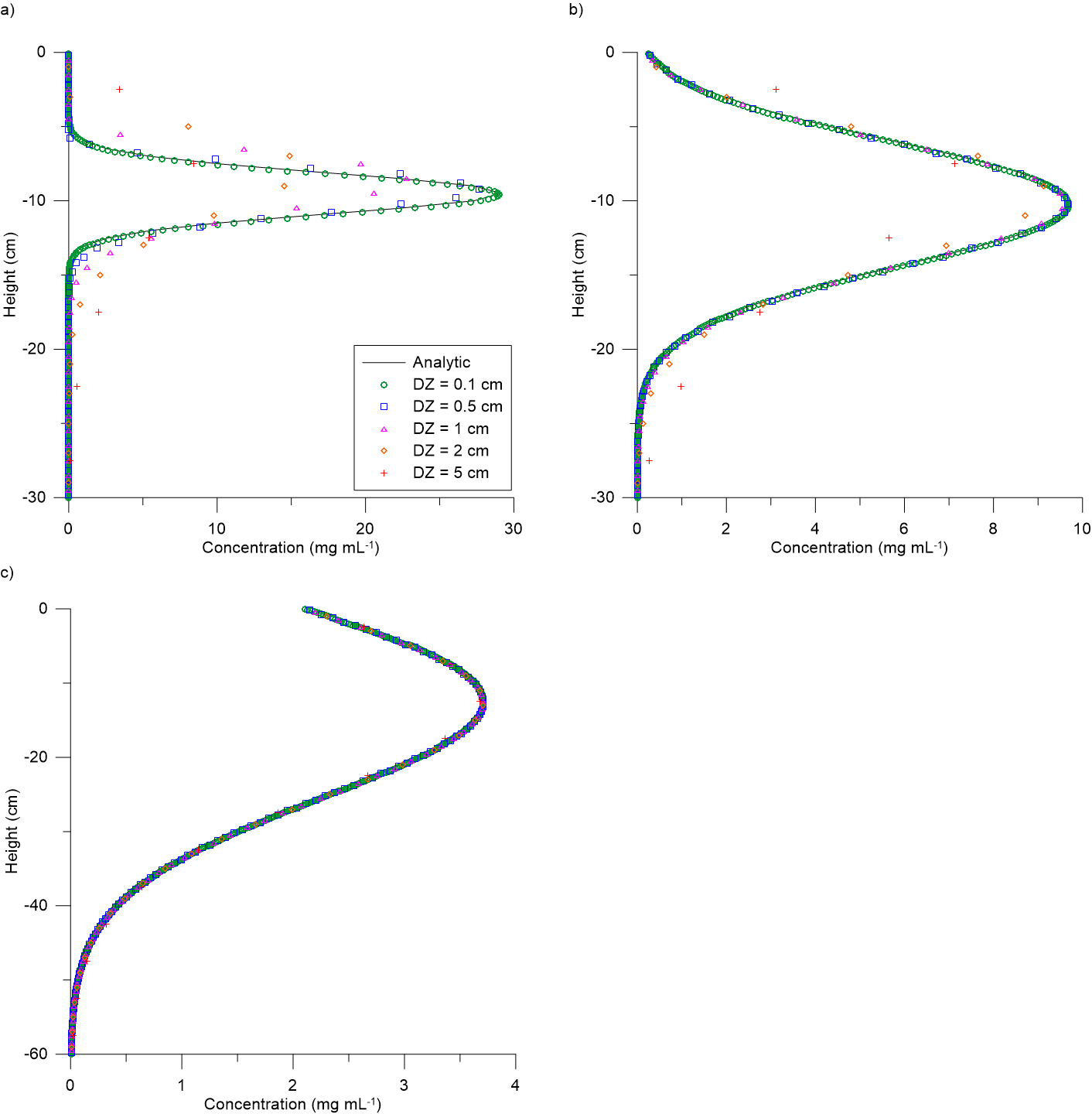
where \(c\) is the solute concentration in the liquid phase (mg mL-1), \(M\) is the areic mass of solute applied during the pulse (mg cm-2), \(\theta\) is the volumetric water content (cm3 cm-3), \(R\) is the retardation factor (-), \(k\) is a decay coefficient (d-1), \(t\) is the time (d), \(v\) is the pore water velocity (cm d-1; \(v\) = \(q/\theta\), with \(q\) the soil water flux density cm3 cm-2 d-1), \(z\) is the soil depth (cm), and \(D\) is the apparent dispersion-diffusion coefficient (cm2 d-1) here with \(D\) = \(vL_{\text {dis}}\), with \(L_{\text {dis}}\) the dispersion length (cm). Here we consider: \(q\) = 0.1 cm3 cm-2 d-1, \(\theta\) = 0.319 cm3 cm-3, \(M\) = 31.9 mg cm-2 (\(c\) of pulse: \(c_0\) = 319 mg mL-1; pulse duration \(t_0\) = 1 d; \(M\) = \(qc_0t_0\)), \(R\) = 1 (no retardation), \(k\) = 0 d-1 (no decay), and three values for \(L_{\text {dis}}\): 0.1 cm, 1 cm, and 10 cm. The soil profile was 200 cm long with uniform soil type (Table 14.4) and different spatial discretizations were used: \(\Delta z\) = 0.1 cm, 0.5 cm, 1 cm, 2 cm and 5 cm. The concentration profile refer to \(t\) = 30 d (Figure 14.2). For the case with a relative high dispersion length (\(L_{\text {dis}}\) = 10 cm) the discretization visibly has no effect on the solute profile in the soil column. However, for a small dispersion length (\(L_{\text {dis}}\) = 0.1 cm) the coarser discretizations result in more flattening of the concentration profile (lower maximum concentration; more flattening at the upper and bottom tails); the case with dispersivity of 1 cm shows an intermediate behaviour. Some statistics are provided in Table 14.5.
Vanderborght and Vereecken (2007) reviewed dispersivities for one-dimensional modelling. The dispersivities reported from field studies were on average several tens of centimetres (up to several hundred centimetres), whereas those for soil cores a small soil columns were about 10 cm or slightly less (in line with an earlier review by Beven et al. (1993). Since most studies with SWAP-WOFOST will be focussing on the field scale, the larger dispersivities will be used, for which in this example no effect of the spatial discretization was observed. In fact, in SWAP the numerical dispersion is taken into account when solving the solute transport equation, thus minimizing the contribution of numerical dispersion.
| h_{ini} (cm) | \(\theta_r\) (cm3 cm-3) | \(\theta_s\) (cm3 cm-3) | \(\alpha\) (cm-1) | \(n\) (-) | \(\lambda\) (-) | \(K_s\) (cm d-1) |
|---|---|---|---|---|---|---|
| -35.5429 | 0.08 | 0.43 | 0.04 | 1.6 | 0.5 | 5 |
| Case | Description | \(r^2\) | RMSE | NRMSE |
|---|---|---|---|---|
| \(L_{dis}\) = 0.1 cm | \(\Delta z\) = 0.1 cm | 0.9973468 | 0.2297944 | 0.2300078 |
| \(\Delta z\) = 0.5 cm | 0.9842242 | 0.5604398 | 0.5604398 | |
| \(\Delta z\) = 1 cm | 0.8331041 | 1.8226638 | 1.8226638 | |
| \(\Delta z\) = 2 cm | 0.6170492 | 2.7548587 | 2.7548334 | |
| \(\Delta z\) = 5 cm | 0.7735463 | 1.1442146 | 1.8264901 | |
| \(L_{dis}\) = 1 cm | \(\Delta z\) = 0.1 cm | 0.9994941 | 0.0576308 | 0.0575579 |
| \(\Delta z\) = 0.5 cm | 0.9993324 | 0.0660819 | 0.0660825 | |
| \(\Delta z\) = 1 cm | 0.9994942 | 0.0648315 | 0.0648249 | |
| \(\Delta z\) = 2 cm | 0.9932554 | 0.2186590 | 0.2185718 | |
| \(\Delta z\) = 5 cm | 0.9200389 | 0.7648084 | 0.7632395 | |
| \(L_{dis}\) = 10 cm | \(\Delta z\) = 0.1 cm | 0.9997694 | 0.0234360 | 0.0234956 |
| \(\Delta z\) = 0.5 cm | 0.9998135 | 0.0220141 | 0.0220142 | |
| \(\Delta z\) = 1 cm | 0.9998195 | 0.0219101 | 0.0219081 | |
| \(\Delta z\) = 2 cm | 0.9998119 | 0.0227732 | 0.0227651 | |
| \(\Delta z\) = 5 cm | 0.9996507 | 0.0390091 | 0.0389218 |
14.4 Infiltration-runoff
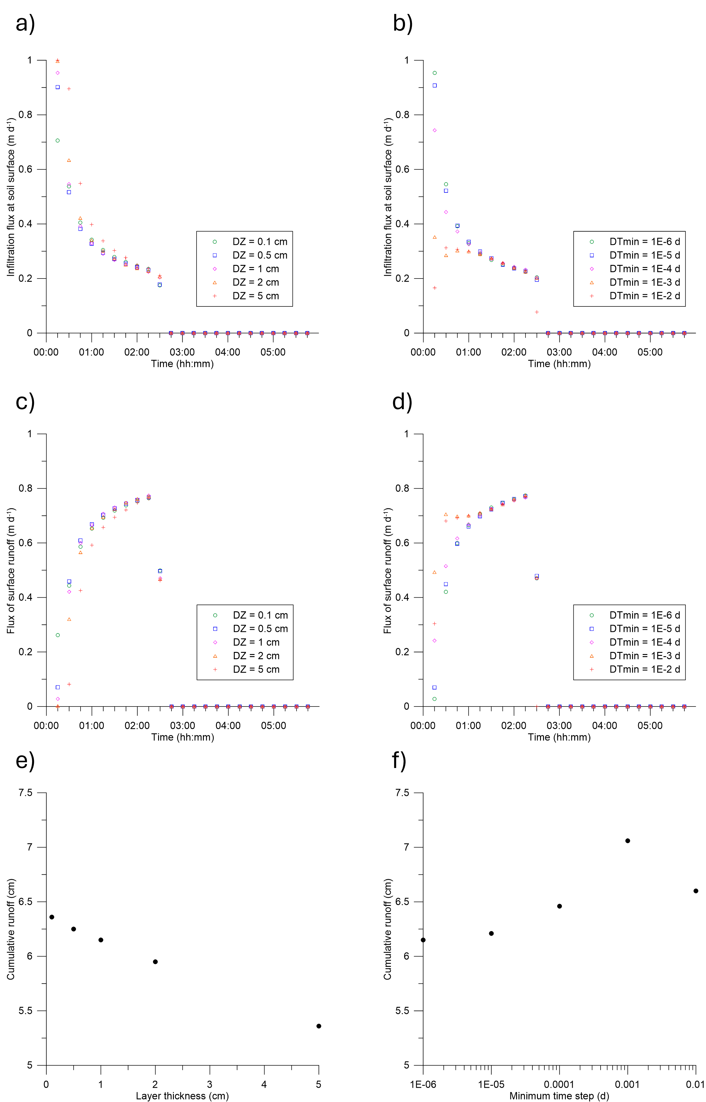
This example is based on one of the default test cases to which each new release of SWAP is tested (based on Van Dam 2000; Van Dam and Feddes 2000). In a uniform soil with uniform pressure head (Table 14.6) a single rain event is considered: 100 mm in 2.4 h (0.1 d). The focus is on the infiltration flux at the soil surface and the amount of runoff. Comparisons are done for different discretizations of the soil column: \(\Delta z\) = 0.1 cm, 0.5 cm, 1 cm, 2 cm and 5 cm (all at \(\Delta t_{\text {min}}\) = 10-6 d); and for different minimum (initial) time steps: \(\Delta t_{\text {min}}\) = 10-6 d, 10-5 d, 10-4, 10-3 and 10-2 d (all at \(\Delta z\) = 1 cm).
The infiltration flux at the soil surface, the flux of runoff at the soil surface and the cumulative runoff for are presented in Figure 14.3: panels a), c) and e) refer to the dependency on spatial discretization, and panels b), d) and f) refer to the dependency on minimum time step. Coarser spatial discretization result in lower predictions of runoff, and larger minimum (initial) time steps result in higher predicted runoff. It should be noted that for the cases \(\Delta t_{\text {min}}\) = 10-4, 10-3 and 10-2 d there were increasing mass balance errors in the calculations.
| h_{ini} (cm) | \(\theta_r\) (cm3 cm-3) | \(\theta_s\) (cm3 cm-3) | \(\alpha\) (cm-1) | \(n\) (-) | \(\lambda\) (-) | \(K_s\) (cm d-1) |
|---|---|---|---|---|---|---|
| -832.5 | 0.01 | 0.43 | 0.0249 | 1.507 | -0.14 | 17.5 |
In addition, the sensitivity of the runoff equation in SWAP can also be analysed analytically. The runoff equation in SWAP is given by
\[ {q_{{\rm{runoff}}}} = \left\{ {\begin{array}{*{20}{c}} 0&{H \le 0}\\ {\frac{{{H_{{\rm{ref}}}}}}{\gamma }{{\left( {\frac{H}{{{H_{{\rm{ref}}}}}}} \right)}^\beta }}&{H > 0} \end{array}} \right. \tag{14.4}\]
where \(H\) is the height of the ponded water layer above the threshold, i.e., \(H\) = \(h_0\) – \(h_{\text {0,threshold}}\), \(H_{\text{ref}}\) is a reference value for \(H\) with \(H_{\text{ref}}\) by definition equal to 1 cm, \(\beta\) is a dimensionless shape parameter which according to Manning’s theory equals 5/3 or approximately 2 (Hillel 1980), and \(\gamma\) is a resistance of water flow over the land surface (d). The presence of the (dummy) variable \(H_{\text{ref}}\) is there to avoid the dimension of \(\gamma\) being a function of the value of \(\beta\).
The sensitivity of this equation for changes (uncertainty) in the magnitude of the contributing parameters can be quantified as follows. The elasticity (\(E\)) is defined as the relative change in function value (\(f\)) divided by the relative change in parameter value (\(p\)), given by
\[ E = \frac{\frac {{\rm{d}}f}{f}}{\frac {{\rm{d}}p}{p}} = \frac {p}{f} \frac{{\rm{d}}f}{{\rm{d}}p} \tag{14.5}\]
A value of \(E\) = +1 means that x% change in parameter \(p\) results in x% change in function value \(f\); for \(E\) < 1 the sensitivity is low, whereas for \(E\) > 1 the sensitivity is high. The elasticity for the runoff equation can be given analytically as follows. The sensitivity to changes in \(H\) (> 0) is given by
\[ E_{\rm{H}} = \beta \tag{14.6}\]
Since \(\beta\) equals about 5/3 to 2, runoff is sensitive to changes in H, which, of course, changes during the simulation. The sensitivity to changes in \(\gamma\) is given by
\[ E_\gamma = - 1 \tag{14.7}\]
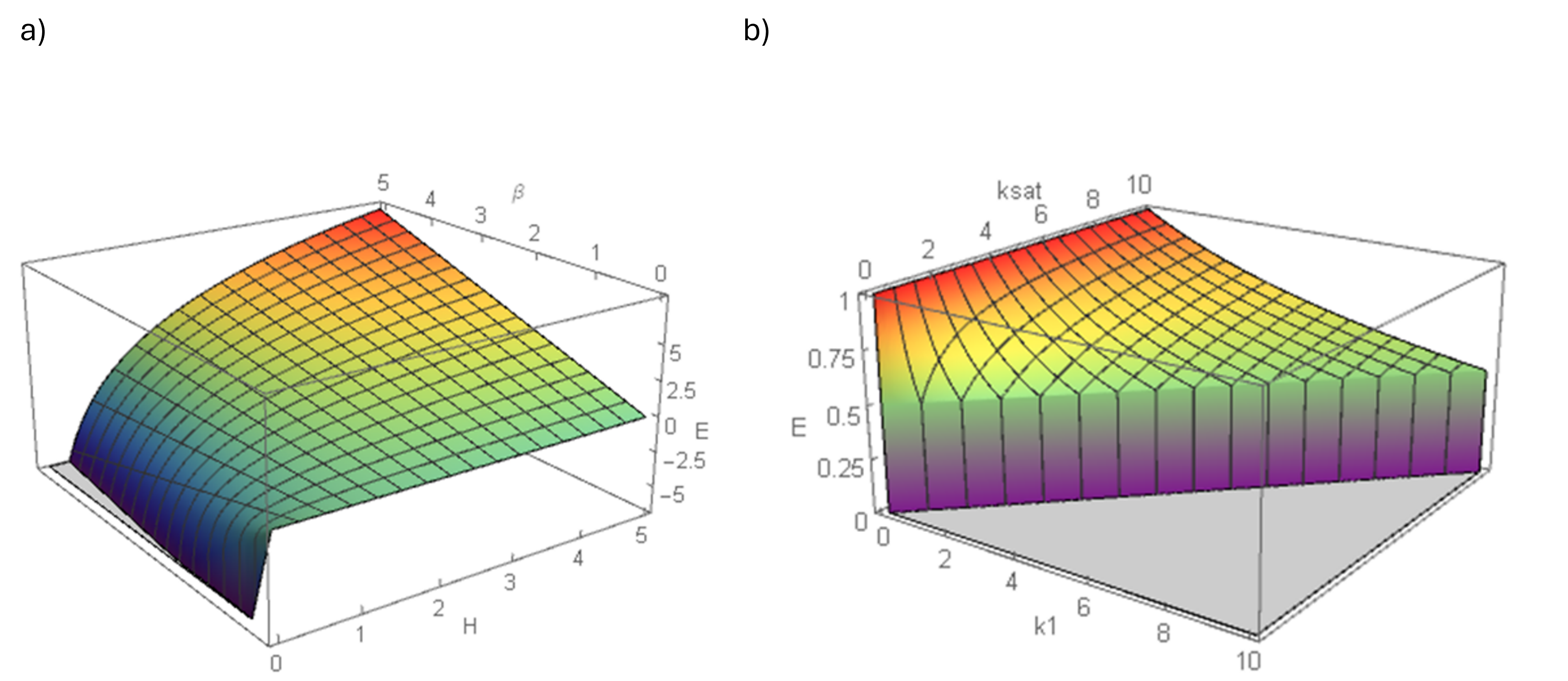
Irrespective of \(H\) and \(\beta\) runoff changes minus the same magnitude as \(\gamma\); e.g. if the resistance increases by 50% runoff will decrease by 50%. The sensitivity to changes in \(\beta\) is given by (Figure 14.4)
\[ {E_\beta } = \beta \ln \left[ {\frac{H}{{{H_{{\rm{ref}}}}}}} \right] \tag{14.8}\]
The sensitivity equals \(\beta\) multiplied by the natural logarithm of \(H\). For \(H\) < \(H_{\text{ref}}\) (\(H\) < 1 cm) this means that runoff decreases with increasing \(H\), and for \(H\) > \(H_{\text{ref}}\) (\(H\) > 1) this means that runoff increases with increasing \(H\); for the special case \(H\) = \(H_{\text{ref}}\) the sensitivity equals zero. Since elasticities of 1 or more are present this means that the parameters \(\beta\) and \(\gamma\) need to be known well.
Since H comprises the actual ponding height (\(h_0\)) and the runoff threshold ponding height (\(h_{\text {0,threshold}}\)) their elasticities are given as well (\(H\) > 0, or \(h_0\) > \(h_{\text {0,threshold}}\)):
\[ {E_{{h_0}}} = \frac{{{h_0}}}{{{h_0} - {h_{\rm{0,threshold}}}}}\beta \tag{14.9}\]
and
\[ {E_{{h_{0,threshold}}}} = - \frac{{{h_{\rm{0,threshold}}}}}{{{h_0} - {h_{\rm{0,threshold}}}}}\beta \tag{14.10}\]
For small values of \(h_{\text {0,threshold}}\) its sensitivity approaches 0, whereas for large values of \(h_{\text {0,threshold}}\) (and small values for \(h_0\) - \(h_{\text {0,threshold}}\)) its sensitivity approaches \(-\beta h_{\text {0,threshold}}\).
14.5 Capillary rise
Van Walsum and Veldhuizen (2011) considered a semi-dynamic case study with focus on the development of a steady-state capillary rise situation (their section 5.4.1). A soil profile (length 550) initially in hydrostatic equilibrium with groundwater level at 100 cm below soil surface is subject to constant evapotranspiration of 3 mm d-1. The grass crop has a constant rooting depth of 30 cm. At 100 cm below soil surface a infiltration drain (resistance 50 d) is present that acts as the source of water. A steady-state condition will develop in course of time. Four conditions differing in spatial discretization was studied by van Walsum and Veldhuizen (2011) which was used here too (Table 14.7). The main focus is on the dynamics that occurs between the infiltrating drain depth (100 cm below soil surface) and the soil surface. Note that for the upper layers (rooting zone) the differences between the four cases is small, and the major differences are seen at depth 50-150 cm.
| Soil depth (cm) | Case 1 (1 cm) | Case 2 (2.5 cm) | Case 3 (5 cm) | Case 4 (variable) |
|---|---|---|---|---|
| 0-5 | 1 | 1 | 1 | 1 |
| 5-35 | 1 | 2.5 | 2.5 | 2.5 |
| 35-50 | 1 | 2.5 | 5 | 5 |
| 50-90 | 1 | 2.5 | 5 | 10 |
| 90-150 | 1 | 2.5 | 5 | 10 |
| 150-550 | 1 | 10 (150-240); 20 (240-300); 50 (300-550) | 10 (150-240); 20 (240-300); 50 (300-550) | 10 (150-200); 20 (200-300); 40 (300-540) |
Figure 14.5 shows the development of the steady-state upward water flux density (capillary rise) at depths 30, 50 and 100 cm and the development of the pressure head at the soil surface (first layer). Table 14.8 shows the differences in at the end of the simulation period (365 d). According to the coarser discretization (Case 4) the capillary rise was highest and actual transpiration was equal to potential transpiration. It required the highest input of water from the infiltrating drain, resulted in the lowest groundwater level. The case with the fine discretization (Case 1) resulted in the lowest actual transpiration (5.2% less that potential transpiration), the lowest input of water from the infiltrating drain (13.7% less than for Case 4), and the highest groundwater level. The steady-state capillary rise equals between 2 and 2.5 mm d-1, which is less than the potential evapotranspiration rate of 3 mm d-1. This difference is partly due to differences in actual transpiration (Table 14.8) and partly due to a great reduction in evaporation at the soil surface (\(E_{\text {act}}\) = 24.3 mm, \(E_{\text {pot}}\) = 202 mm; for all cases). The difference in position of the groundwater level are small. Great differences, however, are seen at the soil surface. Cases 1 and 2 show extremely drying out of the top layer compared to Case 4.
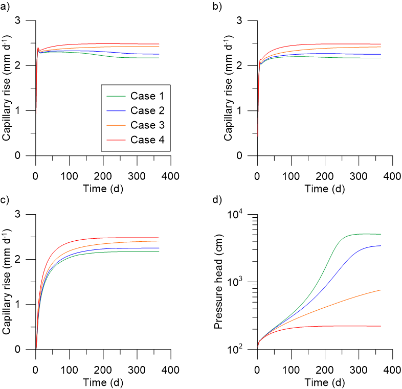
| Case | Actual transpiration (mm) | Groundwater level (cm) | Drain infiltratoin (mm) |
|---|---|---|---|
| Case 1 | 846.6 | 110.9 | 729.8 |
| Case 2 | 867.5 | 111.1 | 753.3 |
| Case 3 | 891.8 | 112.0 | 795.0 |
| Case 4 | 893.0 | 112.4 | 845.6 |
In these calculations normal arithmetic averaging of \(K\) at the layer interfaces was used. When using weighted geometric averaging for Cases 1 and 4 this resulted in very small differences in steady-state capillary rise at depth 30 cm (< 1%). For Case 4 a simulation with \(K\) implicitly included in the numerical solution of the Richards equation resulted in negligible differences.
Kroes et al. (2018) analysed the impact of capillary rise and recirculation of percolation water below grassland, maize and potatoes in Dutch soils. They concluded that soil water and crop growth modelling should consider both capillary rise from groundwater and recirculation of percolation water as this improves the accuracy of yield simulations. Neglecting these processes implies neglecting yield reductions for grassland, maize and potatoes of respectively 26, 3 and 14% or respectively about 3.7, 0.3 and 1.5 t dry matter per hectare and overestimates of groundwater recharge of 17% for grassland and 46% for potatoes, or 63 and 34 mm yr−1, respectively.
14.6 Case study Watervision Agriculture
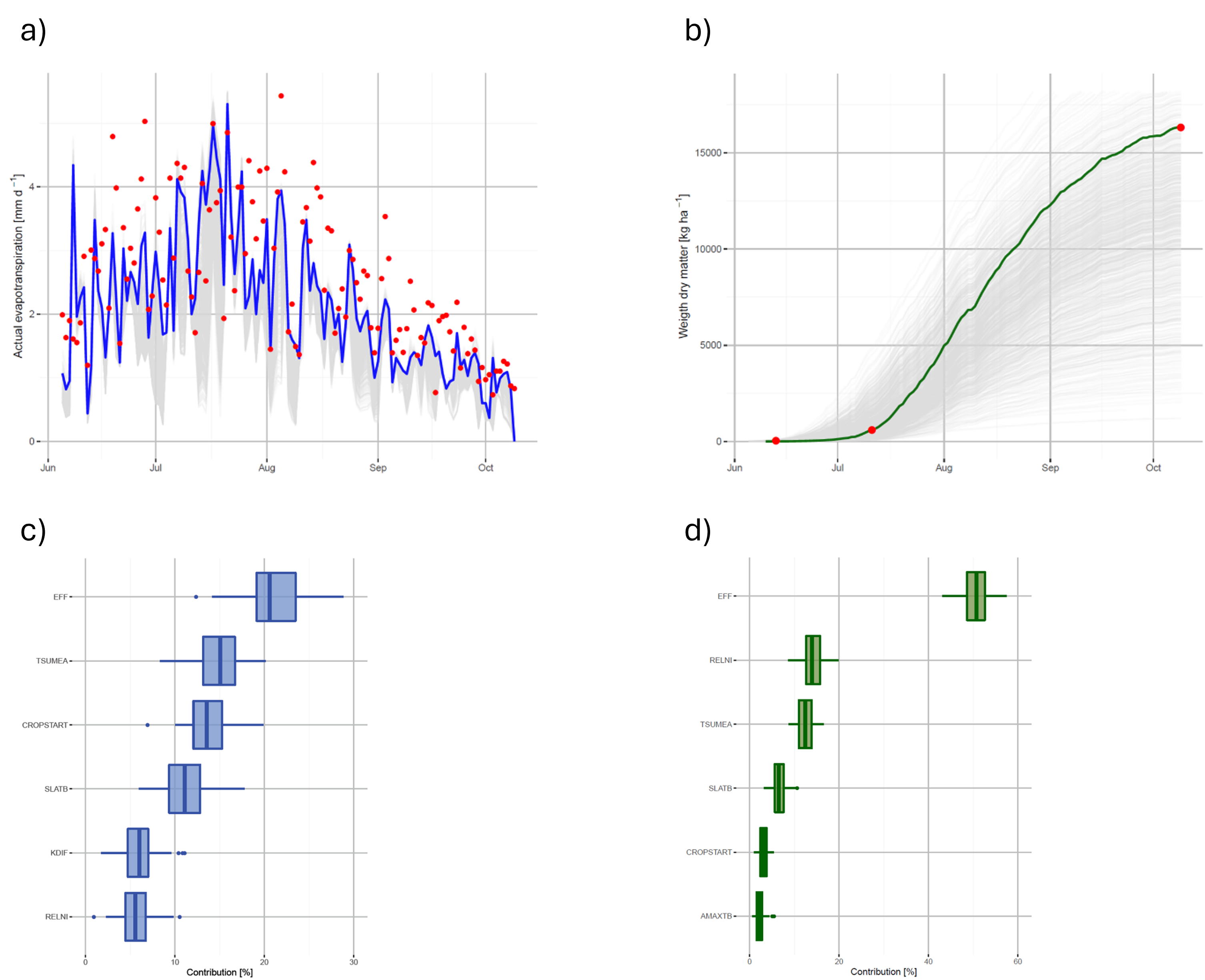
For the project Watervision Agriculture (Dutch: Waterwijzer Landbouw; https://waterwijzerlandbouw.wur.nl/) the following sensitivity analysis was performed (own study, unpublished data). Estimation of actual evapotranspiration and actual crop yield using SWAP-WOFOST is complex. A large number of variables need to be known in order to obtain realistic output. A regression-based sensitivity analysis was performed to identify the uncertainty contribution of input variables and parameters (i.e., those determining \(ET\), CO_2, phenology and stress: nine in total: AMAXTB [max CO2 assimilation rate], EFF [light use efficiency], CFBS [coefficient to convert potential evapotranspiration into potential evaporation], CH [crop height], CROPSTART [starting date of crop growth], KDIF [extinction coefficient for diffuse visible light], RELNI [RELMF; management factor to account for other forms of stress], SLATB [specific leaf are], TSUMEA [temperature sum from emergence to anthesis]) in relation to specific model output (typically \(ET\), \(\theta\) and dry matter production). A Monte-Carlo type analysis was performed assuming parameter probability density functions.
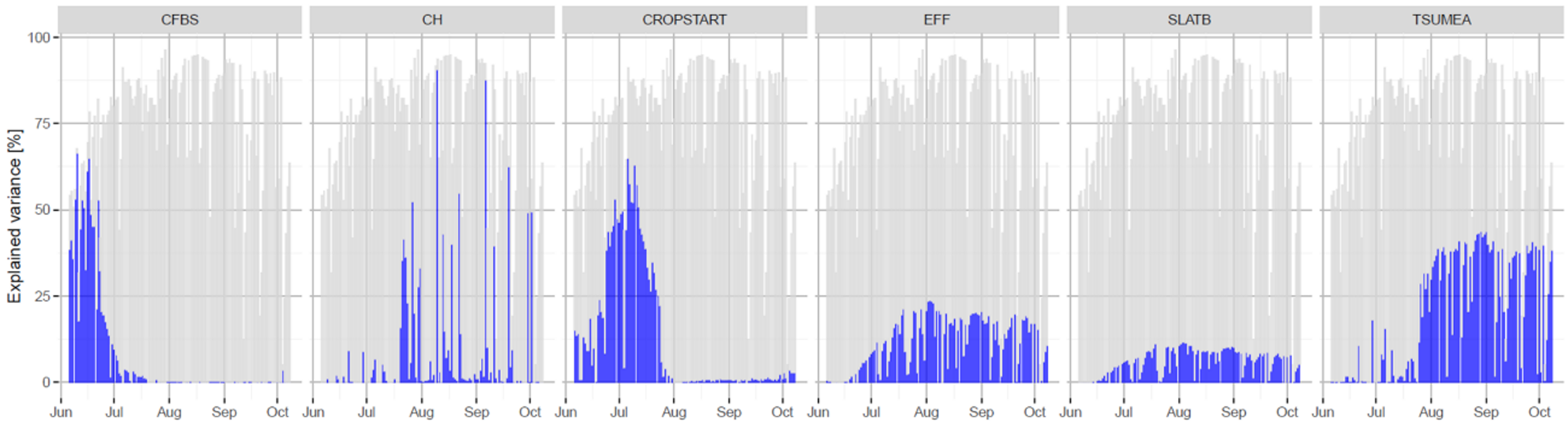
Average annual evapotranspiration was 220 mm with a 95% confidence interval between 180 and 260 mm (Figure 14.6 a). The actual yield was 11250 kg ha-1 with a 95% confidence interval between 6000 and 16000 kg ha-1 (Figure 14.6 b). By linear regression the total percentage of variation accounted for was 85% for ET and 90% for dry matter production. For both \(ET\) and yield the parameter EFF contributed the most to the percentage variance accounted for (Figure 14.6 c,d). Based on a day-to-day application of this method revealed that the sensitivity for the studied parameters differs throughout the season (Figure 14.7).
14.7 SWAP senstivity analyses in literature
In several studies published in the literature sensitivity (or uncertainty) analyses have been reported using the SWAP model. In this chapter some selected studies will be briefly described, and some of the conclusions reported by these authors will be given. For details, the reader is referred to the citations.
14.7.1 Groenendijk et al. (2014)
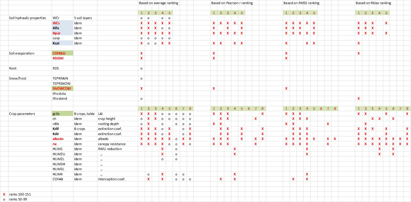
In the GENESIS project (EU FP7; https://cordis.europa.eu/article/id/92657-improved-management-of-groundwater-resources) measured nitrate leaching in a lysimeter was used to perform model comparison between several simulation models, with SWAP being one of the models. Before the actual calibration and validation simulations were done, it was decided to perform a sensitivity analysis (Groenendijk et al. 2014). Based on the soil profile description, the depths at which sensors were installed, the cropping cycles, and measured pressure heads at the bottom of the lysimeter, the SWAP model was parameterized. The major unknowns were the physical properties of the soil layers and some crop growth parameters. A one-at-a-time sensitivity analysis (using the SENSAN module of PEST (Doherty 2005)) was performed for the six Mualem-van Genuchten parameters of the five soil layers, two parameters determining soil evaporation and five parameters determining the effects of frost and snow, the maximum rooting depth, and 14 crop parameters for eight crops (in total 150 parameters). Based on a best initial guess for each of these parameters, they were changed by +10% and by -10%. The objective function was composed of the sum of squared differences between 1461 observed and predicted values of daily seepage water amounts (weight 1.0), and daily water content data at depths 0.35, 0.6, 0.9 and 1.8 m (weight 10.0). For that both the Pearson \(r\) ranking, RMSE (root mean squared error) ranking and bias ranking were calculated, and finally these rankings were averaged. Figure 14.8 shows the obtained outcome of this analysis. From that it was concluded that for later calibration the focus needed to be on the Mualem - Van Genuchten parameters \(θ_s\), \(n\), and \(K_s\) for all five soil layers, one soil evaporation reduction parameter (COFRED), one snowmelt parameter (SNOWCOEF), and for each crop the maximum LAI at harvest. For the two sensitive crop parameters albedo and crop resistance it was decided that default known parameters from the literature would suffice.
14.7.2 Droogers et al. (2008)
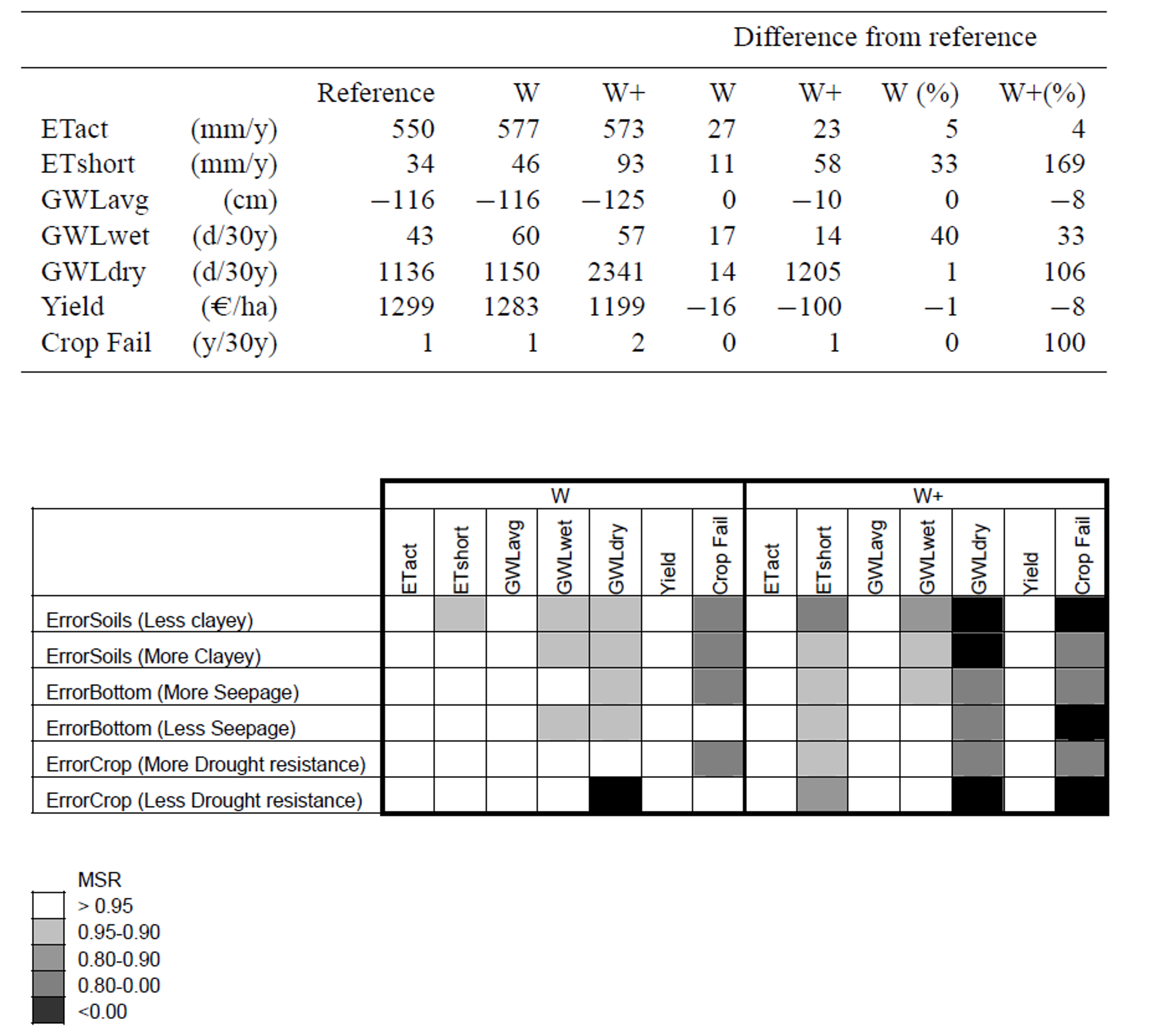
Simulation models are, by definition, approximations of reality. When studying the effects of, e.g., climate change based on model predictions, one could argue that observed effects are due to model errors. To evaluate the impact of model inaccuracy on impact assessment of climate change Droogers et al. (2008) altered the calibrated model to reflect the most common parameter uncertainties. A 10% change was applied to the following parameters: the Mualem-van Genuchten parameters \(\alpha\), \(n\) and \(K_{\text{sat}}\), the average value and amplitude of the bottom water flux density, and the Feddes transpiration reduction parameters \(h_3\) and \(h_4\). The major output variables considered were (averaged over 30 years): actual evapotranspiration (\(ET_{\text{act}}\)), water shortage (\(ET_{\text{short}}\) = \(ET_{\text{pot}}\) - \(ET_{\text{act}}\)), groundwater level (GWL_{}), number of days when GWL (groundwater level) was within 50 cm (GWL_{}) and below 170 cm (GWL_{}), crop yield (Yield), and number of years where crop yield was less than 80% of potential (Crop Fail). To express the impact of model inaccuracy versus the impact of the scenario itself, they introduced the Model-Scenario-Ratio (MSR) measure for their evaluation. “The value of MSR indicates to what extent the impact of a scenario contributes to the final findings compared to model inaccuracy. An MSR value of 1 indicates that the model inaccuracy doesn’t play a role and results are a function of the scenario only. An MSR value of 0 indicates that the response of the impact assessment originates for 50% from the changing climate scenario, and 50% from an inherent model uncertainty. MSR values lower than zero indicate that responses are dominated by model inaccuracy rather than by the scenario evaluated.”
Their analysis focussed on the impact of climate scenarios W and W+ compared to reference climate. Their results are summarized in Figure 14.9.
They concluded that:
- for the two climate scenarios an increase in water shortage, more extremes in wet and dry periods, and a small reduction in agriculture production can be expected
- for the W scenario the MSR analysis indicated that model inaccuracy was not relevant for most indicators
- for the W+ scenario (enhanced drought conditions) model inaccuracy plays a role for some indicators. However, > 90% of the assessed impact could still be attributed to the scenario itself and not to model inaccuracy.
14.7.3 Stahn et al. (2017)
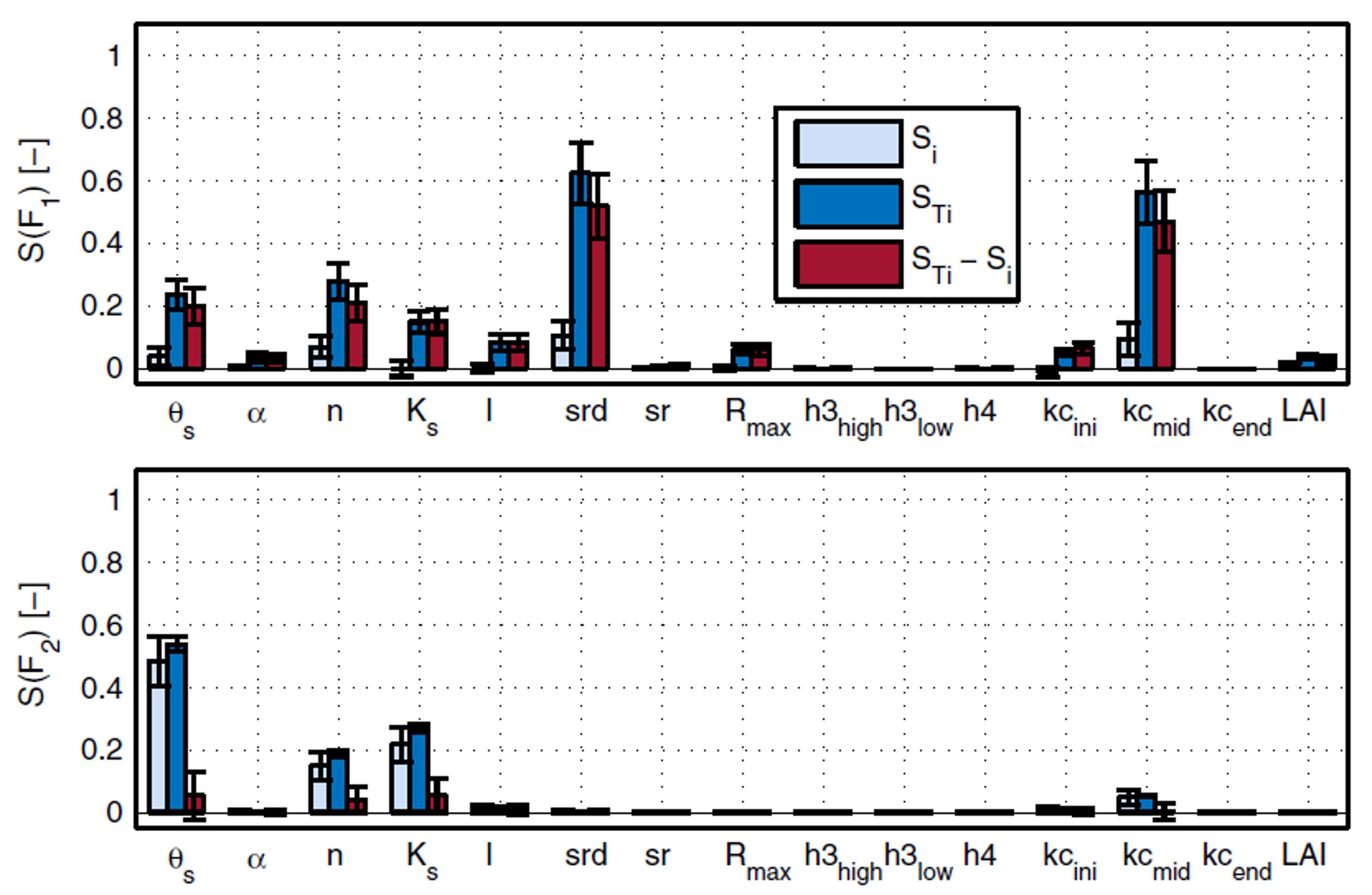
Stahn et al. (2017) performed a global Sobol variance-based sensitivity analysis for SWAP (version 3.2.36). Details of the method employed can be found in the paper. In total 15 parameters were considered: five parameters for the Mualem-van Genuchten soil hydraulic properties (\(θ_s\), \(n\), \(\alpha\), \(\lambda\), \(K_s\)), three rooting distribution parameters (\(srd\) [shape parameter for exponential root distribution], \(sr\) [shape parameter for logistic root depth increase, \(Rmax\) [maximum rooting depth]), three transpiration reduction parameters of the Feddes function (\(h_{3,high}\), \(h_{3,low}\), \(h_4\); determining drought stress), three crop coefficients (\(K_{c,ini}\), \(K_{c,mid}\), \(K_{c,end}\)) and \(LAI\). The sensitivity was performed with focus on simulated volumetric water contents and soil pressure heads (compared to measurements at depths 30 and 60 cm). High sensitivities were observed for parameters \(srd\), \(K_{c,mid}\), \(n\), \(\theta_s\) and \(K_s\) (in that order) when considering their effects on volumetric water content; for pressure head these were \(\theta_s\), \(K_s\), \(n\) and \(K_{c,mid}\) (in that order) (Figure 14.10). The most sensitive parameters were later optimized using a calibration procedure. For the none-sensitive parameters the authors stated: “It cannot be expected that information on the overall insensitive parameters (\(h_{3,high}\), \(h_{3,low}\), \(h_4\), \(sr\) and \(k_{c,end}\)) would be provided by the observational data. Therefore, these parameters were excluded from optimisation by fixing them to experience values.”
The authors summarized and concluded with (some quotes):
- Mixed cropping was effectively represented in the model [SWAP] structure.
- These results demonstrate how complex and variable the relationship between parameters and model outputs can be in simulation models such as SWAP and underline the necessity of conducting a global sensitivity analysis to detect such patterns.
- These findings underline once again the need of considering multiple data types in parameter optimisation in order to constrain the resulting solutions to describe different model outputs simultaneously well.
- The results showed that most of the parameters are well identified, independent of the level of parameter interaction. However, interactions seem to be relevant for parameter identifiability.
14.7.4 Wanders et al. (2012)
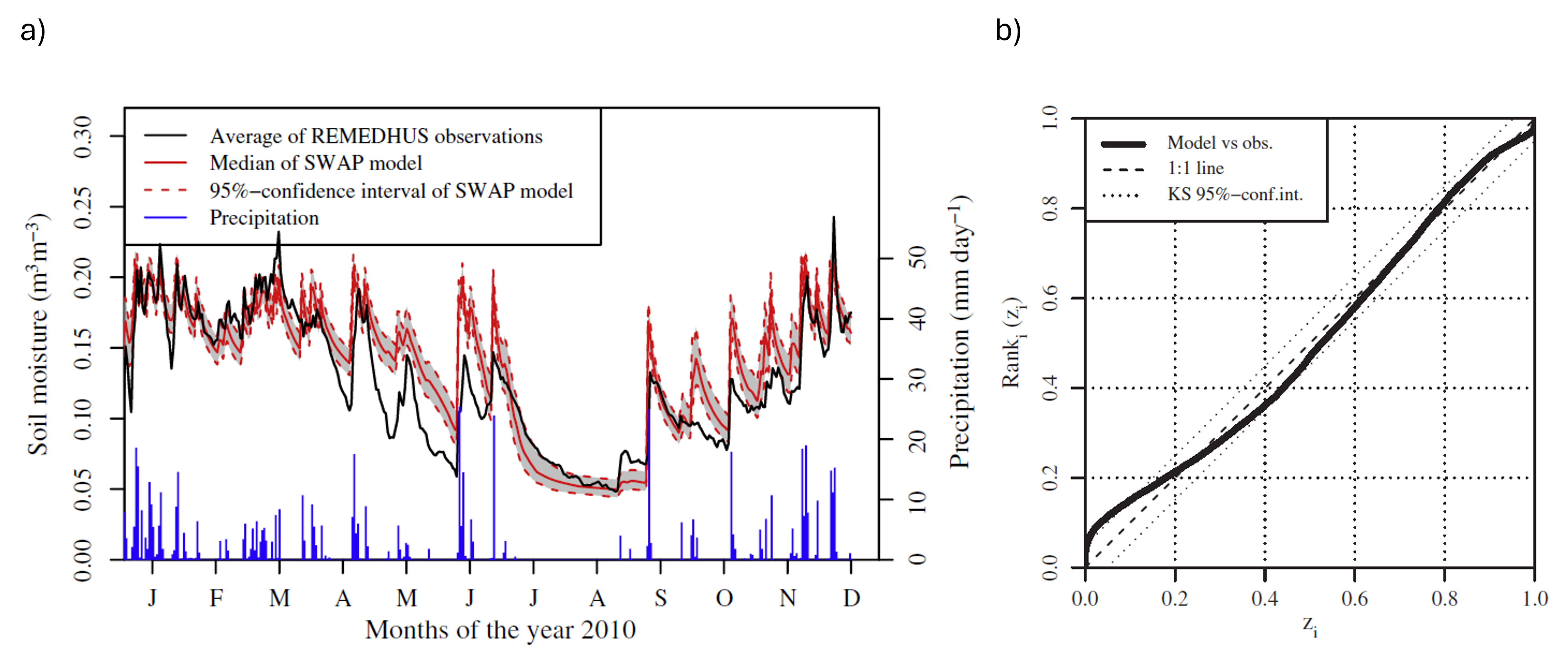
Wanders et al. (2012) performed a Monte-Carlo-type sensitivity analysis using SWAP to determine the 95% confidence interval of predicted soil moisture at 5 cm depth and compared this with measured soil moisture contents for a test site in central Spain. The following parameters were used in their sensitivity analysis: the Mualem-van Genuchten parameters \(\theta_r\), \(\theta_s\), \(\alpha\), \(n\), \(K_s\), the meteorological input variables precipitation and evapotranspiration, and the crop leaf are index. No detailed information on the probability density functions for these parameters were provided. For the year 2010 a good agreement between modelled and observed water contents (with a slight positive bias equal to 0.01 m3 m-3), with a narrow 95% confidence interval around the modelled results (Figure 14.11 a). For the months May and June the model slightly over-estimated the observations, which according to the authors was “probably caused by an underestimation of evapotranspiration.” They also presented this comparison in a so-called QQ-plot (Figure 14.11 b). The predictive QQ-plot is a measure to check whether the obtained Monte Carlo simulation results in a probability density function (PDF) that corresponds to the PDF of the model prediction errors. “The predictive QQ-plot … shows that the modeled soil moisture is within the 95%-confidence interval of the Kolmogorov–Smirnov test (KS-test). The bias of 0.01 m3 m-3 … was also found in the predictive QQ-plot. The SWAP model slightly overestimates the amount of low soil moisture values compared to the observations as seen from a small deviation below 0.2 m3 m-3 soil moisture content. This deviation is however not significant as shown by the KS-test.”
This study does not provide quantitative data on which parameters are more sensitive and which others are less sensitive. Instead, it provides more insight in the uncertainty of model predictions for given uncertainty of several model parameters.
14.8 Resume
The analysis presented in this chapter is not meant to provide a universal sensitivity analysis of the SWAP-WOFOST model. It provides some insight in the model’s sensitivity for a few case studies. The following general remarks are given:
- It should be a good modelling practice to perform a sensitivity analysis at the start of a modelling project. As each project may have its own focus, so may be the sensitivity analysis different from study to study.
- The heart of the SWAP model is formed by the numerical solution of the (non-linear) partial differential equations describing water movement and solute transport. Since it generally known that solving these equation numerically are dependent on the chosen spatial and temporal discretization, one should consider these as important.
- There is no unique way to perform a sensitivity analysis. One can choose from screening methods (often used for models with a large number of input variables; e.g. the one-at-a-time method, several factorial methods, Cotter’s method), local sensitivity analysis (often based on analytical partial derivatives; not always possible), and global sensitivity analysis (e.g. Monte-Carlo analysis, response surface methodology, Fourier amplitude sensitivity test). Sections Section 14.7.1 and Section 14.7.2 provided an example of the one-at-a-time screening method, and sections Section 14.6 and Section 14.7.3 provided examples of global sensitivity analyses.
- Water movement in porous media is highly determined by the non-linear soil physical hydraulic properties. Therefore it is likely that SWAP is sensitive to the parameters that determine these properties (see Section 14.7.1, Section 14.7.3).
- Crop production is determined by the environmental driving variables (radiation, temperature, CO2), but is also determined by transpiration. Transpiration is determined by the availability of water in the root zone. Therefore, crop growth is dependent on parameters that drive these processes (see example in Section 14.6, Section 14.7.2, Section 14.7.3).