13 Verification and validation
13.1 Comparison with analytical solutions
The core of SWAP is the numerical solution of the non-linear partial differential equation (the so-called Richards equation) describing water movement in porous media. In order to verify whether or not the numerical solution in SWAP is correctly implemented it is useful to compare SWAP simulations with analytical solutions. However, since the Richards equation is a non-linear partial differential equation, analytical solutions are scarce, and often require specific constitutive relationships. By default SWAP uses the Mualem (1976) – van Genuchten (1980) constitutive relationship describing the non-linear relations between volumetric water content, pressure head and hydraulic conductivity. For these situations no analytical solution are known. Analytical solutions can be produced in case these relationships are of exponential form. In the following we compare analytical transient infiltration profiles from the literature in which the water retention characteristic is given by
\[ S = \frac{{\theta - {\theta _{\rm{r}}}}}{{{\theta _{\rm{s}}} - {\theta _{\rm{r}}}}} = \exp \left( {\alpha h} \right) \tag{13.1}\]
and the hydraulic conductivity function is given by
\[ K = \exp \left( {\alpha h} \right) \tag{13.2}\]
The differential moisture capacity \(C = {\text d}\theta/{\text d}h\) is also needed in SWAP and follows easily from Equation 13.1: \(\alpha (\theta_s - \theta_r){\text {exp}}(\alpha h)\). For this purpose the SWAP code was temporarily adapted such that the Mualem- van Genuchten calculated \(\theta\), \(K\) and \(C\) were overruled by these exponential relations. Best results were obtained when the SWAP option to include K implicitly in the solution procedure was used. For this purpose also the derivative \({\text d}K/{\text d}h\) needs to be known, which follows from Equation 13.2 as \(\alpha {\text {exp}}(\alpha h)\).
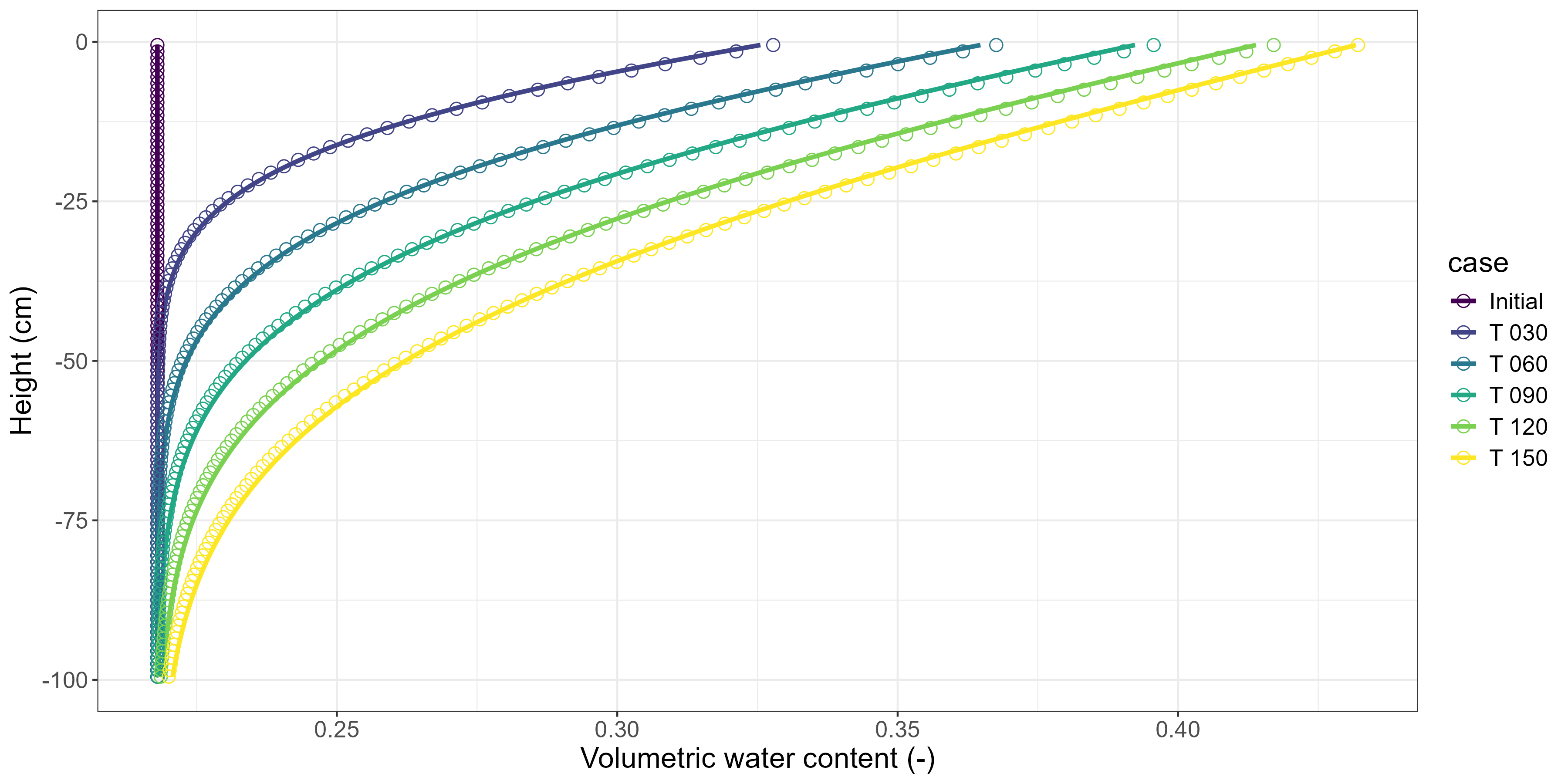
The first example is from Basha (1999) where infiltration in a uniform dry soil can be calculated up to the time of ponding. The parameter settings of Basha (1999) were slightly adapted such that the time of ponding (also available as an analytical solution) occurred exactly at 150 min. Figure 13.1 shows the excellent comparison between SWAP simulations and the analytical solution.
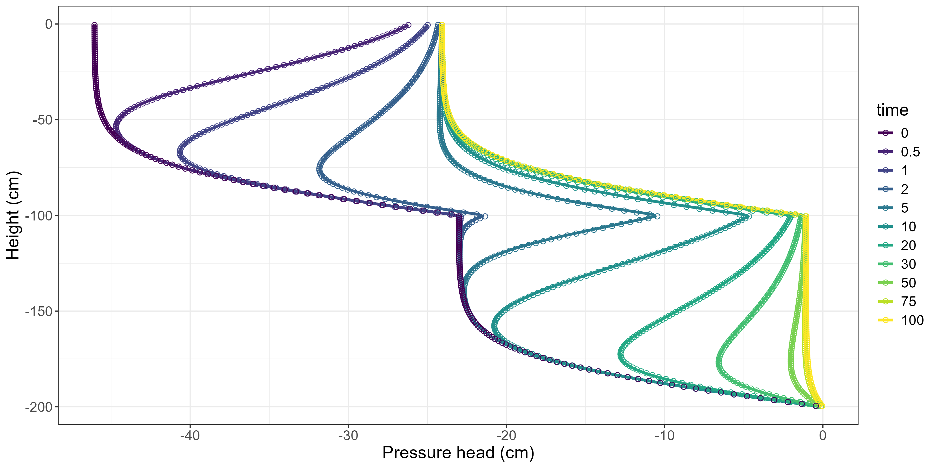
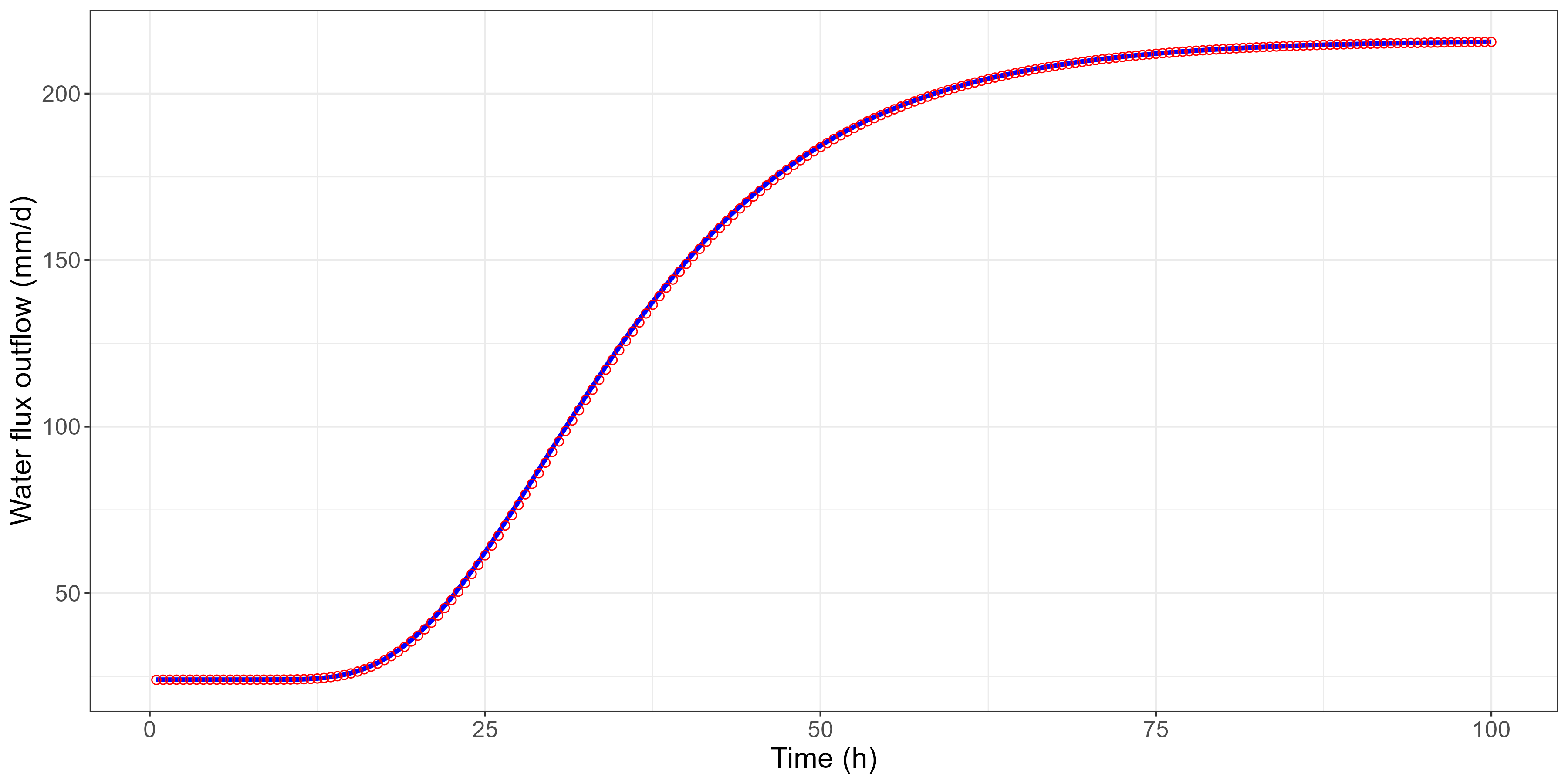
The second example refers to infiltration into a layered soil as provided by Srivastava and Yeh (1991), using their parameter settings. Also here the SWAP simulations for \(h(z)\) (Figure 13.2) and the outflow rate at the bottom of the soil column (Figure 13.3) are equal to the analytical solutions.
13.2 WOFOST
WOFOST (World Food Studies; Boogaard et al. (2014)) is a stand-alone model to predict potential and water-limited crop production (available at: https://www.wur.nl/en/Research-Results/Research-Institutes/Environmental-Research/Facilities-Products/Software-and-models/WOFOST.htm). The Fortran version of WOFOST 7.1 is embedded in the SWAP Fortran code, where specific changes were implemented needed for the two-way interaction between SWAP and WOFOST. For example, the internal water balance in WOFOST is no longer used as the transpiration reduction is now calculated by SWAP and transferred to WOFOST where it may result in reduced crop growth. Vice versa, the leaf are index calculated by WOFOST is exchanged with SWAP where it is used to divide evapotranspiration in transpiration and evaporation.
WOFOST is one of the well-known Wageningen crop growth models by the school of C.T. de Wit. All these Wageningen models follow the hierarchical distinction between potential and limited production, and share similar crop growth sub models, with light interception and CO2 assimilation as growth driving processes, and crop phenological development as growth controlling process.
The major developments in WOFOST will be monitored. The development team of WOFOST has decided to change from the Fortran language to Python, so that the maintenance of the Fortran code is likely no longer guaranteed. Since WOFOST is based on generally accepted crop growth modelling theories by the school of C.T. de Wit, it is not likely that major changes in performance of WOFOST can be expected.
In order to verify that the implementation of WOFOST embedded in the SWAP Fortran code can reproduce the results of the standalone WOFOST version a set of pre-defined test cases are used (de Wit et al. (2019); https://github.com/ajwdewit/pcse/tree/master/tests/test_data). The reference set has been generated for 11 locations across Europe and covers 7 different crops which leads to 44 unique test cases since not all crops are cultivated on all locations. Only the potential crop growth is considered since the water-limited crop growth is depending on hydrological soil moisture conditions calculated by SWAP.
For all situations the potential crop production predicted by SWAP-WOFOST is identical to that obtained with the stand-alone WOFOST model. This verifies proper implementation of the WOFOST code in SWAP.
13.3 Examples of validation
Some say a simulation model is never validated enough or is never completely validated. This is typically the case for models that deal with a great diversity of aspects (processes) and parameters, like in SWAP. Furthermore, comparison of model predictions with field data is not always possible in an objective way, since it is unlikely that field experiments are performed such that all required model input data are known/measured. The current standard set of test cases against which each new SWAP release is tested contains a few cases where field data are available for comparison with simulated data. These will be briefly illustrated below.
13.3.1 Cranendonck
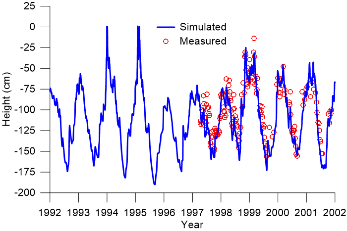
Growth of forage maize on sandy soil, well fertilized with N (no official reference; Joop Kroes, pers. comm.). For maize we used the standard WOFOST crop file for maize. The soil consisted of 60 cm topsoil (zand-B2; Wösten, Veerman, and Stolte (1994)) with a zand-O2 subsoil (290 cm; Wösten, Veerman, and Stolte (1994)), with a free drainage bottom boundary condition. KNMI weather data from stations 370 (Eindhoven) and 918 (Maarheze; rainfall) were used. Figure 13.4 shows the good correspondence between measured and simulated groundwater levels.
13.3.2 Wildenborch
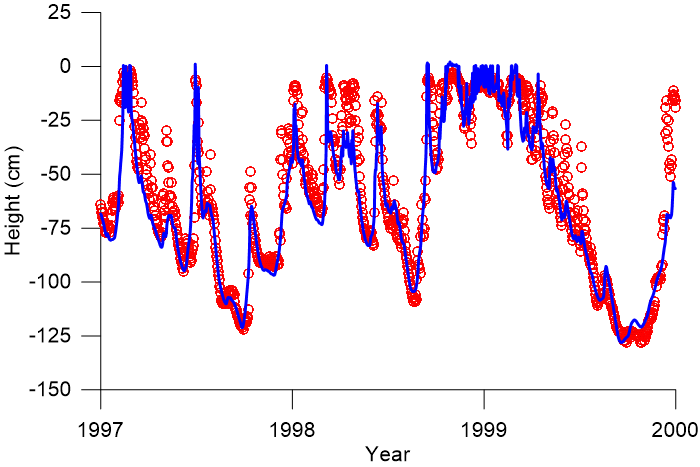
This study was described by Massop et al. (2001) and the simulation was reported in van Dam et al. (2008). This study refers to a case with use of the extended drainage option in SWAP. For this purpose the internal simple grass growth option was used. The soil profile consisted of zand-B1 (0-25 cm; Wösten et al. (2001)) and zand-O1 (25-405 cm; Wösten et al. (2001)). A flux-type bottom boundary condition was used which followed from a hydraulic head of an underlying aquifer and a vertical resistance of a separating aquitard. Figure 13.5 shows the good correspondence between measured and simulated groundwater levels.
13.3.3 Castricum
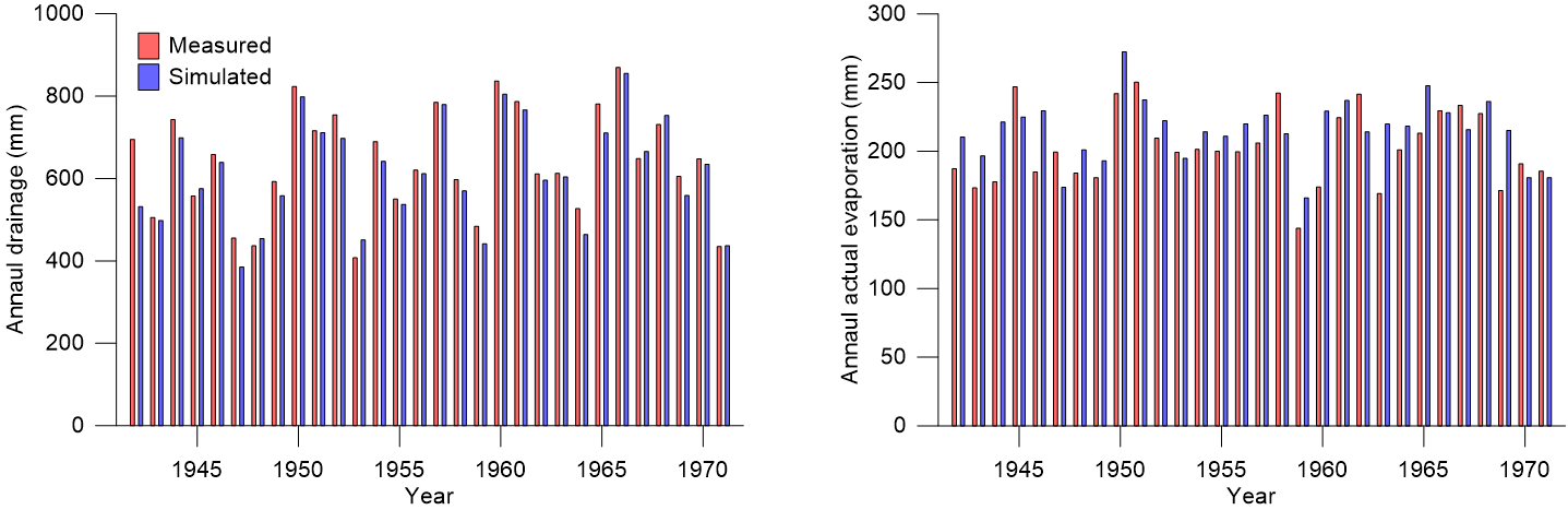
From a lysimeter experiment in Castricum the yearly amount of drainage and actual evaporation from bare soil was used to compare with SWAP simulations; description of and data from the lysimeter study was described in van der Hoeven (2011). The soil profile consisted of 0-35 cm zand-B1 and 35-250 cm zand-O1 (Wösten, Veerman, and Stolte 1994). A constant groundwater level at 225 cm below soil surface was used as bottom boundary condition. Local weather data were used. Figure 13.6 shows the good correspondence between measured and simulated drainage and evaporation.
13.3.4 Zegveld
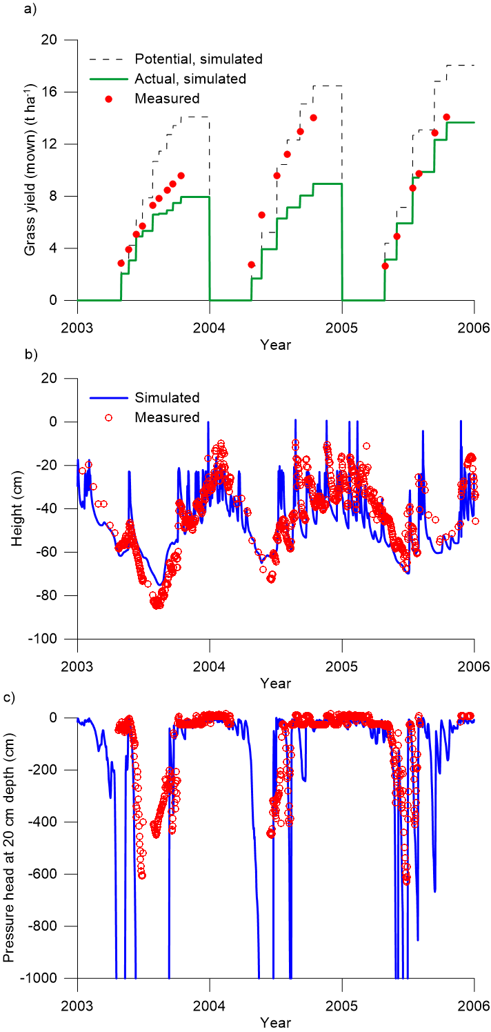
The Zegveld case refers to a wet grassland on peat with simple drainage (R. Hendriks, pers. comm.; see also Kroes et al. (2015)). A flux-type bottom boundary condition was used which followed from a hydraulic head of an underlying aquifer and a vertical resistance of a separating aquitard. Figure 13.7 shows the correspondence between measured and simulated yields, groundwater levels and pressure head at 20 cm depth. Since this test case was included as a reference test case, the input variables have not been changed so that such changes do not interfere with possible changes in simulation result with each new release of SWAP. In a separate study (Kroes et al. 2015) optimized the input data to obtain better correspondence between measured and simulated yields (Figure 13.8).

13.3.5 Rusthoeve
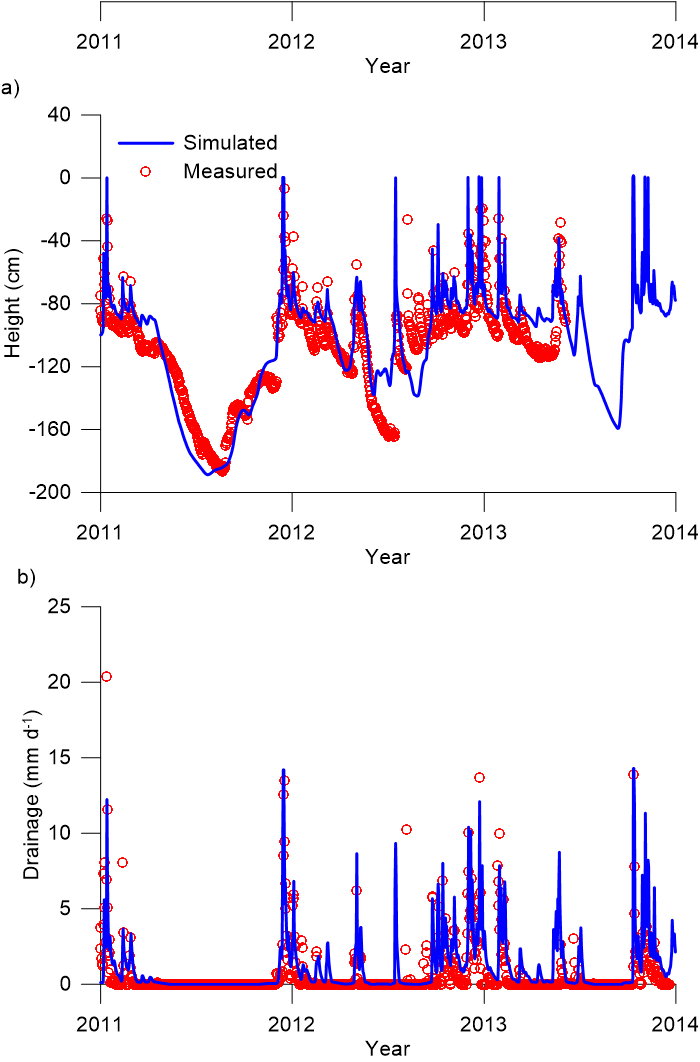
The Rusthoeve case was described in Schipper et al. (2015) (their case ‘blok7’). Three different crops were considered: sugar beet (2011), winter wheat (2011-2012) and potatoes (2013). The soil profile was 0-25 cm zavel-B9, 25-45 cm zavel-O10 and 45-545 cm zavel-O9 (Wösten, Veerman, and Stolte 1994). A flux-type bottom boundary condition was used which followed from a hydraulic head of an underlying aquifer (measured, tabulated data) and a vertical resistance of a separating aquitard. Two drainage levels were considered: at 90 cm (drain tube distance 6 m, drain resistance 66 d) and at 130 cm (drain tube distance 100 m, drain resistance 2500 d). KNMI weather data from stations 310 (Vlissingen) and 755 (Kortgene; rainfall) were used.
Only for the last crop (potatoes) the yield was measured as 8.6 t ha-1, which was well simulated by the model: 8.7 t ha-1. Figure 13.9 shows the good correspondence between measured and simulated groundwater level and drain discharge.
13.3.6 Dijkgraaf
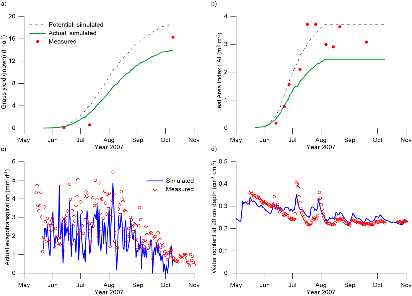
The Dijkgraaf case is based on Elbers et al. (2010). The main crop was maize (end of May until beginning of October 2007) simulated as a default WOFOST crop. The remainder of the year the soil was covered by grass (simple grass growth option in SWAP). The soil profile was 0-25 cm zand-B2 (2001) and 25-300 cm zand-O2 (2001). A flux-type bottom boundary condition was used which followed from a hydraulic head of an underlying aquifer (sine function) and a vertical resistance of a separating aquitard. No lateral drainage was considered. Locally measured meteo data of Haarweg was used. Figure 13.10 shows the correspondence between measured and simulated crop data (yield, LAI), actual evapotranspiration, and volumetric water content at 20 cm depth.
13.3.7 Texel
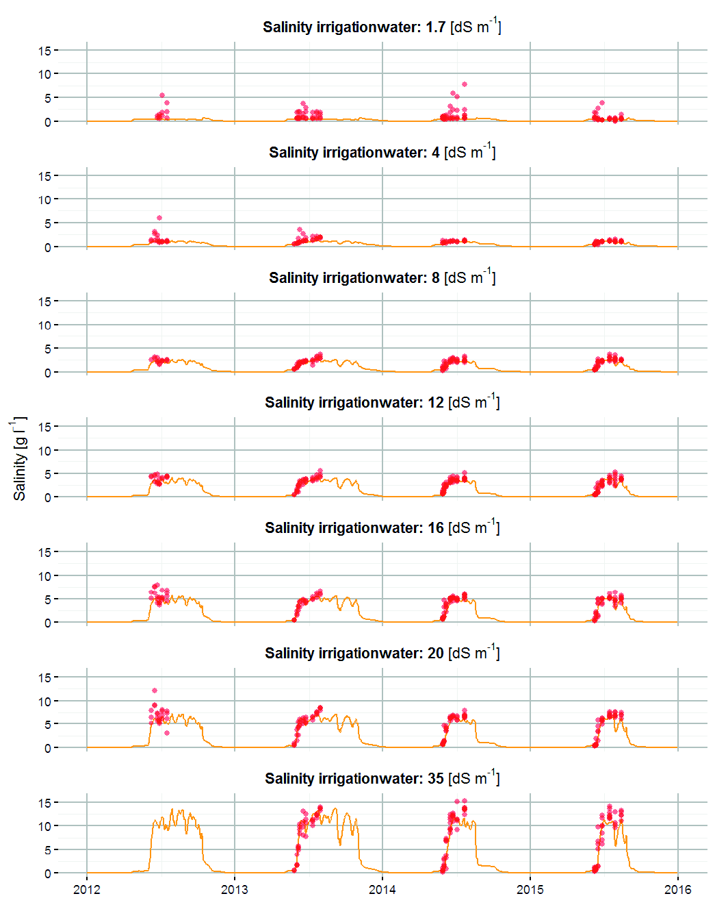
Mulder et al. (2018) validated SWAP-WOFOST for salinity stress in irrigated potatoes. Figure 13.11 shows an example of the good correspondence between simulated and measured salinity in the soil for the different irrigation salinity treatments.
13.4 Applications in literature
SWAP has been used extensively in scientific literature, where it is used either with or without comparison to field data or where it is used in a comparison against other models. On the website https://swap.wur.nl/ a detailed list of literature is given, divided in the following subject areas:
- General reference to SWAP
- On the use of SWAP
- Soil water flow
- Evapotranspiration
- Irrigation management
- Drainage conditions
- Surface water management
- Plant growth
- Soil water extraction by roots
- Soil moisture indicators for natural vegetation
- Salinization
- Solute transport
- Soil water flow as affected by soil spatial heterogeneity
- Sensitivity analysis
- Regional analysis
- Integration with other models
13.5 Resume
The main core of SWAP is the numerical solution of the governing partial differential equation for water movement in porous media. It requires information on the (highly) non-linear, constitutive relationships between the pressure head, volumetric water content and hydraulic conductivity (i.e. water retention and hydraulic conductivity characteristics). SWAP is set-up such that the user (modeller) needs to provide information on soil properties and to define proper initial and boundary conditions. How good the simulation results obtained with SWAP are, depends on these input data. Verification and validation tests are helpful in getting confidence in the SWAP model. In Section 13.1 a SWAP simulation was verified against a transient analytical solution for infiltration in a layered soil, showing that the technical numerical implementation of the solution of the partial differential equation is valid. Such tests have also been performed for solute transport and soil temperature (Heinen, Dik, and Cruijsen 2021). Comparing SWAP simulations with measured field data can be seen as validation. In Section 3.2 seven examples are provided in which comparison is done on groundwater levels, drainage and evaporation from a lysimeter, yield (grass including cuttings; maize), pressure head or volumetric water content at a certain depth, drain discharge, actual evapotranspiration, and salinity of the pore water at a certain depth. Other than for the comparison with analytical solutions, such validation experiments mostly don’t show an exact agreement between simulated and measured data. Then the focus is more on agreement in trends and order of magnitude. SWAP is used extensively in studies reported in scientific literature for a wide range of subjects (see Section 13.4). These can also be seen as examples of validation.