Hupsel Brook
The Hupsel Brook catchment has been a well-known field site for hydrological studies since the 1960s. It has been used for studies on evapotranspiration (Stricker and Brutsaert 1978), soil physical properties (Hopmans and Stricker 1989), relations between flow routes and water quality (Van den Eertwegh 2002; Rozemeijer et al. 2010; Van der Velde et al. 2012) and rainfall-runoff modelling (Bierkens and Puente 1990; Brauer 2014). The catchment of 6.5 km2 is slightly sloping (0.8%). Its soil consists of a loamy sand layer (with some clay, peat and gravel) of 0.2 to 10 m thickness on an impermeable clay layer of more than 20 m thickness (Brauer 2014).
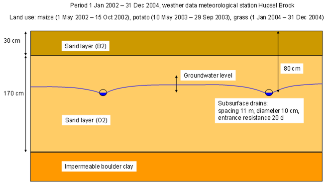
We selected a typical field in the Hupsel Brook catchment to demonstrate SWAP in- and output files. Figure 12.1 shows the environmental settings. The simulation run covers the period 2002-2004 with 3 crops: maize, potato and grass. Each crop is simulated with a different crop module in SWAP: maize with the simple module for a static crop, potato with the WOFOST module for a dynamic crop, and the modified WOFOST module for grass growth.
Potential evapotranspiration fluxes are calculated with daily meteorological observations and the Penman-Monteith equation. Also, daily values for rainfall are used, as in the catchment with its mild slopes and sandy soils no runoff is expected. The sandy soil profile consists of a top- and sublayer with thicknesses of 30 and 170 cm, respectively. The soil hydraulic functions are derived from the Staring series (Heinen, Bakker, and Wösten 2020): texture B2 for the top layer and texture O2 for the sublayer.
At the bottom of the soil profile, a layer of boulder clay with low permeability prevents vertical soil water movement. Therefore, at the bottom, a zero flux condition is specified. Drainage fluxes are calculated for subsurface drains at 80 cm depth and with a lateral distance of 11 m.
Initial soil water contents are assumed to be in hydrostatic equilibrium with a groundwater level at 75 cm depth. On 5 January 2002, a tracer is applied, which leaches in the subsequent years towards the drains.
The SWAP simulation can be run using a batch file (run_swap.cmd), which refers to the SWAP executable and the main input file, see Section 1.4. SWAP can print two yearly water balances: a summary (*.bal) and an extensive (*.blc). Tip 12.1 shows an example of the extensive water balance for the year 2002.
* Project:       hupsel
* File content:  detailed overview of water balance components (cm)
* File name:     result.blc
* Model version: SWAP 4.3.1
* Generated at:  2026-06-30 09:54:29

Period             :  2002-01-01  until  2002-12-31
Depth soil profile :  200.00 cm
=================================================+=================================================
INPUT                                            | OUTPUT
                   PLANT    SNOW    POND    SOIL |                   PLANT    SNOW    POND    SOIL
=================================================+=================================================
Initially Present           0.00    0.00   75.19 | Finally present            0.00    0.00   78.01
Gross Rainfall     84.18                         |
Nett Rainfall               0.00   79.93         | Nett Rainfall     79.93
Gross Irrigation    2.40                         |
Nett Irrigation                     2.40         | Nett Irrigation    2.40
                                                 | Interception       4.25
Snowfall                    0.00                 |
Snowmelt                            0.00         | Snowmelt                   0.00
                                                 | Sublimation                0.00
SSDI                                        0.00 | Plant Transpiration                       34.73
                                                 | Soil Evaporation                  11.99
Runon                               0.00         | Runoff                             0.03
Inundation                          0.00         |
Infiltr. Soil Surf.                        77.35 | Infiltr. Soil Surf.               77.35
Exfiltr. Soil Surf.                 7.04         | Exfiltr. Soil Surf.                        7.04
Infiltr. subsurf.                                | Drainage
- system 1                                  0.00 | - system 1                                32.76
Upward seepage                              0.00 | Downward seepage                           0.00
=================================================+=================================================
Sum                86.58    0.00   89.37  152.54 | Sum               86.58    0.00   89.37  152.54
=================================================+=================================================
Storage Change              0.00    0.00    2.82
Balance Deviation   0.00    0.00    0.00    0.00
===================================================================================================
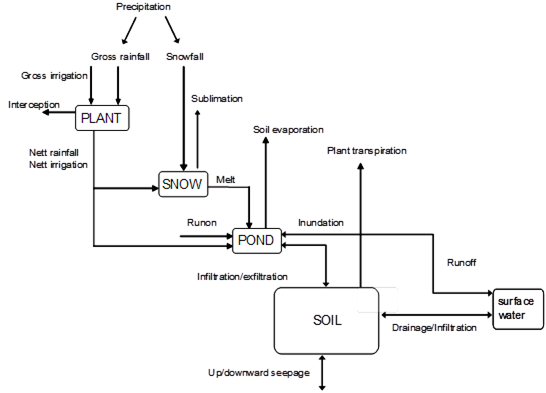
In this output file, the fluxes are presented between the subdomains plant, snow, pond layer, soil, and their environment, as depicted in Figure 12.2. In addition to the in- and outgoing fluxes, of each subdomain also the water storage and balance is depicted. For instance, the ponding layer received 79.93 cm rain, 2.40 cm irrigation and 7.04 cm soil water from the first soil compartment. Of this amount, 11.99 cm evaporated towards the atmosphere and 77.35 cm infiltrated into the first soil compartment. Surface runoff was minimal, amounting to only 0.03 cm. As both the initial and final storage of the ponding layer are zero, the storage change is also zero.
SWAP allows users to define a set of output variables to be written to a file, so that all results can be collected in a single output file (see for additional information Appendix A). For this case study, we aim to generate model outputs for all components of the water and solute balances, along with additional variables related to evapotranspiration (such as potential fluxes and reduction of the potential fluxes due to stress), groundwater levels, and solute concentrations at each depth (see Tip 12.2).
* Part 4: Output files
...

* Specific CSV output file with timeseries (default: no)
 SWCSV = 1    ! Switch, output of variables to be specified
              ! 0 = No csv output
              ! 1 = Regular csv output
              ! 2 = Regular csv output + output of simulation characteristics
              ! 3 = Binary csv output + output of simulation characteristics

 INLIST_CSV = 'WATBAL,ETTERMS,SOLBAL,GWL,C'
Output intervals may range from 0.001 day to 1 year. In this case, output is requested at the end of each month (swmonth = 1). SWAP prints both incremental and cumulative water balance fluxes. Tip 12.3 shows the incremental water fluxes for the year 2002. The actual transpiration rates are close to the potential transpiration rates due to the high rain amounts in the summer season and the shallow groundwater levels. In May, the maize is not yet covering the soil and the actual soil evaporation rate is substantial: 2.47 cm month-1. Drainage mainly occurs in the winter months January – March and October – December. In the summer months May and June the soil water storage declines with 2.50 and 6.78 cm, respectively. Due to large rainfall amounts in July, the soil water storage increases with 2.47 cm. At the monthly resolution, the simulated groundwater levels fluctuate between -34.5 cm (31 December) and -162.9 cm (30 September) with respect to soil surface.
* Project:       hupsel
* File content:  specified output data of SWAP
* File name:     result_output.csv
* Model version: SWAP 4.3.1
* Generated at:  2026-06-30 09:54:29
* (yyyy-mm-dd)  (cm)  (cm)   (cm) (cm)  (cm)  (cm) (cm)  (cm)  (cm)  (cm)  (cm)    (cm)   (cm)   (cm)  (cm)   (cm) ...
DATE            RAIN IRRIG RUNOFF  EIC   EPD  EPOT EACT  TPOT  TACT   DRN  SSDI     GWL PD_VOL IC_VOL  WTOT  DSTOR ...
2001-12-31      0.00  0.00   0.00 0.00  0.00  0.00 0.00  0.00  0.00  0.00  0.00  -75.00   0.00   0.00 75.19   0.00 ...
2002-01-31      4.26  2.40   0.00 0.00  0.00  0.29 0.29  0.00  0.00  5.40  0.00  -65.81   0.00   0.00 76.15   0.96 ...
2002-02-28     12.29  0.00   0.00 0.00  0.00  0.84 0.84  0.00  0.00 10.58  0.00  -52.95   0.00   0.00 77.03   0.88 ...
2002-03-31      3.56  0.00   0.00 0.00  0.00  2.02 1.66  0.00  0.00  4.22  0.00  -79.33   0.00   0.00 74.70  -2.32 ...
2002-04-30      4.21  0.00   0.00 0.00  0.00  3.29 1.71  0.00  0.00  1.02  0.00  -65.18   0.00   0.00 76.19   1.48 ...
2002-05-31      5.29  0.00   0.00 0.08  0.00  4.63 2.47  1.44  1.44  3.79  0.00  -85.96   0.00   0.00 73.69  -2.50 ...
2002-06-30      4.89  0.00   0.00 0.86  0.00  2.08 1.25  9.56  9.56  0.00  0.00 -133.79   0.00   0.00 66.91  -6.78 ...
2002-07-31     14.19  0.00   0.00 1.40  0.00  0.85 0.85  9.47  9.47  0.00  0.00 -149.63   0.00   0.00 69.37   2.47 ...
2002-08-31      6.18  0.00   0.00 0.83  0.00  0.91 0.91  7.39  7.39  0.00  0.00 -143.08   0.00   0.00 66.42  -2.95 ...
2002-09-30      4.05  0.00   0.00 0.64  0.00  0.72 0.72  5.38  5.38  0.00  0.00 -162.90   0.00   0.00 63.74  -2.68 ...
2002-10-31      9.18  0.00   0.00 0.44  0.00  0.71 0.71  1.48  1.48  0.00  0.00 -130.22   0.00   0.00 70.28   6.55 ...
2002-11-30      7.38  0.00   0.00 0.00  0.00  0.42 0.42  0.00  0.00  1.85  0.00  -73.52   0.00   0.00 75.39   5.11 ...
2002-12-31      8.70  0.00   0.03 0.00  0.00  0.15 0.15  0.00  0.00  5.90  0.00  -34.55   0.00   0.00 78.01   2.62 ...
...
On 5 January 2002 a tracer is applied (48 mg cm-2). Tip 12.4 lists the simulated solute balance fluxes for the year 2002. After one year, 9 mg cm-2 solutes have leached towards the drains. The remaining amount, 39 mg cm-2 or 81.1 % of the applied dose, is still in the soil profile and groundwater on 31 December 2002.
* Project:       hupsel
* File content:  specified output data of SWAP
* File name:     result_output.csv
* Model version: SWAP 4.3.1
* Generated at:  2026-06-30 09:54:29
* (yyyy-mm-dd) ... (mg/cm2) (mg/cm2) (mg/cm2) (mg/cm2) (mg/cm2) (mg/cm2) ...
DATE           ...  S_RAIN   S_IRRIG    S_DRN    S_UPT   S_STOT  S_DSTOR ...
2001-12-31     ...    0.00      0.00     0.00     0.00     0.00     0.00 ...
2002-01-31     ...    0.00     48.00     0.00     0.00    48.00    48.00 ...
2002-02-28     ...    0.00      0.00     1.68     0.00    46.32    -1.68 ...
2002-03-31     ...    0.00      0.00     0.89     0.00    45.43    -0.89 ...
2002-04-30     ...    0.00      0.00     0.27     0.00    45.16    -0.27 ...
2002-05-31     ...    0.00      0.00     1.62     0.00    43.54    -1.62 ...
2002-06-30     ...    0.00      0.00     0.00     0.00    43.54     0.00 ...
2002-07-31     ...    0.00      0.00     0.00     0.00    43.54     0.00 ...
2002-08-31     ...    0.00      0.00     0.00     0.00    43.54     0.00 ...
2002-09-30     ...    0.00      0.00     0.00     0.00    43.54     0.00 ...
2002-10-31     ...    0.00      0.00     0.00     0.00    43.54     0.00 ...
2002-11-30     ...    0.00      0.00     1.09     0.00    42.45    -1.09 ...
2002-12-31     ...    0.00      0.00     3.49     0.00    38.96    -3.49 ...
...
Tip 12.5 list the simulated solute concentrations for each soil compartment. When output intervals exceed one day, as in this case, the data represent the conditions at the end of each day. Note that these values reflect the state at the specified date and time and are not averaged over the output interval.
* Project:       hupsel
* File content:  specified output data of SWAP
* File name:     result_output.csv
* Model version: SWAP 4.3.1
* Generated at:  2026-04-09 09:54:29
* (yyyy-mm-dd) ...    (mg/cm3 w)    (mg/cm3 w)    (mg/cm3 w)    (mg/cm3 w)    (mg/cm3 w)    (mg/cm3 w)    (mg/cm3 w)    (mg/cm3 w)    (mg/cm3 w) ...
DATE           ... S_CONC[-0.50] S_CONC[-1.50] S_CONC[-2.50] S_CONC[-3.50] S_CONC[-4.50] S_CONC[-5.50] S_CONC[-6.50] S_CONC[-7.50] S_CONC[-8.50] ...
2001-12-31     ...       0.00000       0.00000       0.00000       0.00000       0.00000       0.00000       0.00000       0.00000       0.00000 ...
2002-01-31     ...       1.41148       1.66137       1.90870       2.16442       2.43420       2.71415       2.99515       3.26867       3.52906 ...
2002-02-28     ...       0.09130       0.10963       0.12995       0.15247       0.17735       0.20476       0.23483       0.26767       0.30337 ...
2002-03-31     ...       0.16595       0.14575       0.13776       0.13870       0.14615       0.15838       0.17418       0.19277       0.21369 ...
2002-04-30     ...       0.05906       0.07055       0.08281       0.09584       0.10963       0.12419       0.13950       0.15557       0.17243 ...
2002-05-31     ...       0.10418       0.09739       0.09934       0.10531       0.11306       0.12163       0.13099       0.14115       0.15242 ...
2002-06-30     ...       0.09769       0.09633       0.11061       0.12829       0.14610       0.16639       0.19005       0.21783       0.25061 ...
2002-07-31     ...       0.01404       0.01698       0.02037       0.02429       0.02881       0.03399       0.03994       0.04676       0.05454 ...
2002-08-31     ...       0.02152       0.01936       0.01932       0.02091       0.02363       0.02716       0.03132       0.03608       0.04149 ...
2002-09-30     ...       0.01323       0.01293       0.01466       0.01723       0.02026       0.02379       0.02787       0.03245       0.03760 ...
2002-10-31     ...       0.00410       0.00442       0.00527       0.00635       0.00752       0.00881       0.01029       0.01197       0.01389 ...
2002-11-30     ...       0.00136       0.00158       0.00190       0.00225       0.00264       0.00308       0.00358       0.00415       0.00479 ...
2002-12-31     ...       0.00037       0.00044       0.00052       0.00062       0.00073       0.00086       0.00100       0.00117       0.00136 ...
...
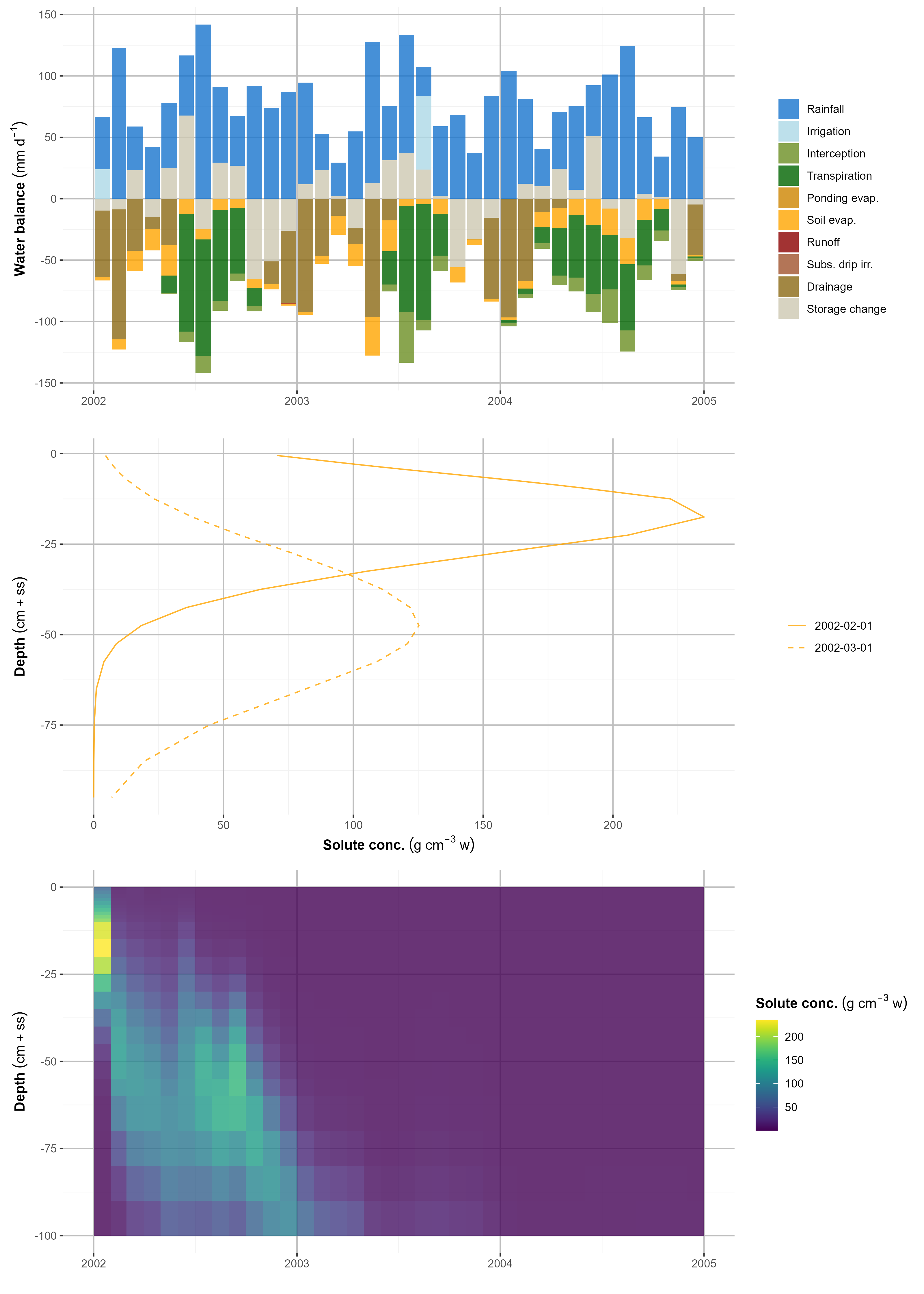
The SWAP download also includes the R-package SWAPtools, which can be used to visualize model results. An example is provided that produces a figure with three panels, an overview of all water balance terms, salinity concentration profiles at the end of January and February, and a time-depth plot of the salinity concentration. This figure can be generated by double-clicking the file plot_swap.cmd and should resemble Figure 12.3. The layout and settings of the figure are defined in control_plot.inp.
Grass growth
This case describes growth of grassland and was used by Kroes and Supit (2011) to study the effects of increasing salinity of groundwater, drought and water excess on grass production in The Netherlands. One field of Ruurlo was selected to show the method and some of the options to simulate growth of grassland. It is a field with high fertilization of 600 kg ha-1 N. Meteorological data are a combination of rainfall from a local weather station and other data (radiation, temperature, windspeed and humidity) from an automatic Dutch national weather station De Bilt (KNMI).
Grass growth is initiated when a temperature sum of 200°C is exceeded. Growth parameters are similar to arable and grassland crops. Management has a separate section in the input file (Tip 12.6). This grassland management section in the input file has 3 parts:
- Part 1: General: in this part the sequence of grass growth is defined: mowing, grazing and/or dewooling has to be chosen.
- Part 2: Grazing settings: this part defines the grazing amount, timing and uptake of livestock.
- Part 3: Mowing settings: this part defines timing and thresholds for mowing.
**********************************************************************************

*** GRASSLAND MANAGEMENT SECTION ***

**********************************************************************************
* Part 1: General

* Define sequence of periods with Grazing (= 1), Mowing (= 2) and Grazing with dewooling (=3) within calender year
* Make sure you have enough periods; last period should continue until the end of the year
  SEQGRZMOW = 2 2 2 2 2 2 2 2 2 2 2 2 2 2 2 2 2 2 2 2

* Switch for timing harvest, either for mowing or grazing
  SWHARVEST = 1              ! 1 = Use dry matter threshold
                             ! 2 = Use fixed dates

* In case of fixed dates (SWHARVEST=2), specify harvest dates (maximum 999):
  DATEHARVEST =
  2004-05-15 2004-06-15 2004-07-15 2004-08-15 2004-09-30
* End of table

**********************************************************************************

**********************************************************************************
* Part 2: Grazing settings (this part is valid when SEQGRZMOW(i)=1 or SEQGRZMOW(i)=3)

* List threshold of above ground dry matter [0..3d5 kg DM/ha, R] to trigger grazing as function of daynumber [1..366 d, R]:
*  DAYNR  DMGRZ
  DMGRZTB =
 152.0 2400.0
 244.0 1800.0
 366.0 1800.0
* End of table

  MXGDGRZ = 28               ! Maximum growing period after harvest [1..366 -, I]

* In case of grazing specify:
  DMRESTGRZ = 700.0          ! Minimum amount of above ground DM after grazing [0..5000 kg DM/ha, R]

* In case of grazing with dewooling (SEQGRAZMOW(i)=3), specify:
  DMRESTDEW = 850.0          ! Remaining yield above ground after dewooling event [0..5000 kg DM/ha, R]

* Grazing event settings:
  DAYGRZ = 4                 ! Maximum days of grazing [1..366 d, I]
  UPTGRZ = 340.0             ! Daily dry matter uptake by grazing [0..2500 kg/ha DM, R]
  LOSSGRZ = 85.0             ! Daily dry matter loss during grazing due to droppings and treading [0..2500 kg/ha DM, R]

* Switch for extra losses due to insufficient pressure head during grazing:
  SWLOSSGRZ = 0              ! 0 = No losses
                             ! 1 = Losses due to treading

**********************************************************************************

**********************************************************************************
* Part 3: Mowing settings (this part is valid when SEQGRAZMOW(i)=2)

* List threshold of above ground dry matter [0..3d5 kg DM/ha, R] to trigger mowing as function of daynumber [1..366 d, R]:
*  DAYNR  DMMOW
  DMMOWTB =
 120.0 4700.0
 213.0 2700.0
 366.0 2700.0
* End of table

  MXGDMOW = 42               ! Maximum growing period after harvest [1..366 -, I]

* In case of mowing always specify:
  DMRESTMOW = 700.0          ! Remaining yield above ground after mowing event [0..5000 kg DM/ha, R]

* Switch for extra losses due to insufficient pressure head during mowing:
  SWLOSSMOW = 0              ! 0 = No losses
                             ! 1 = Losses due to work-ability

* Relation between dry matter harvest [0..3d5 kg/ha, R] and days of delay in regrowth [0..366 d, I] after mowing
  DELAYMOWTB =
    0.0 2.0
 3000.0 3.0
 5000.0 4.0
* End of table
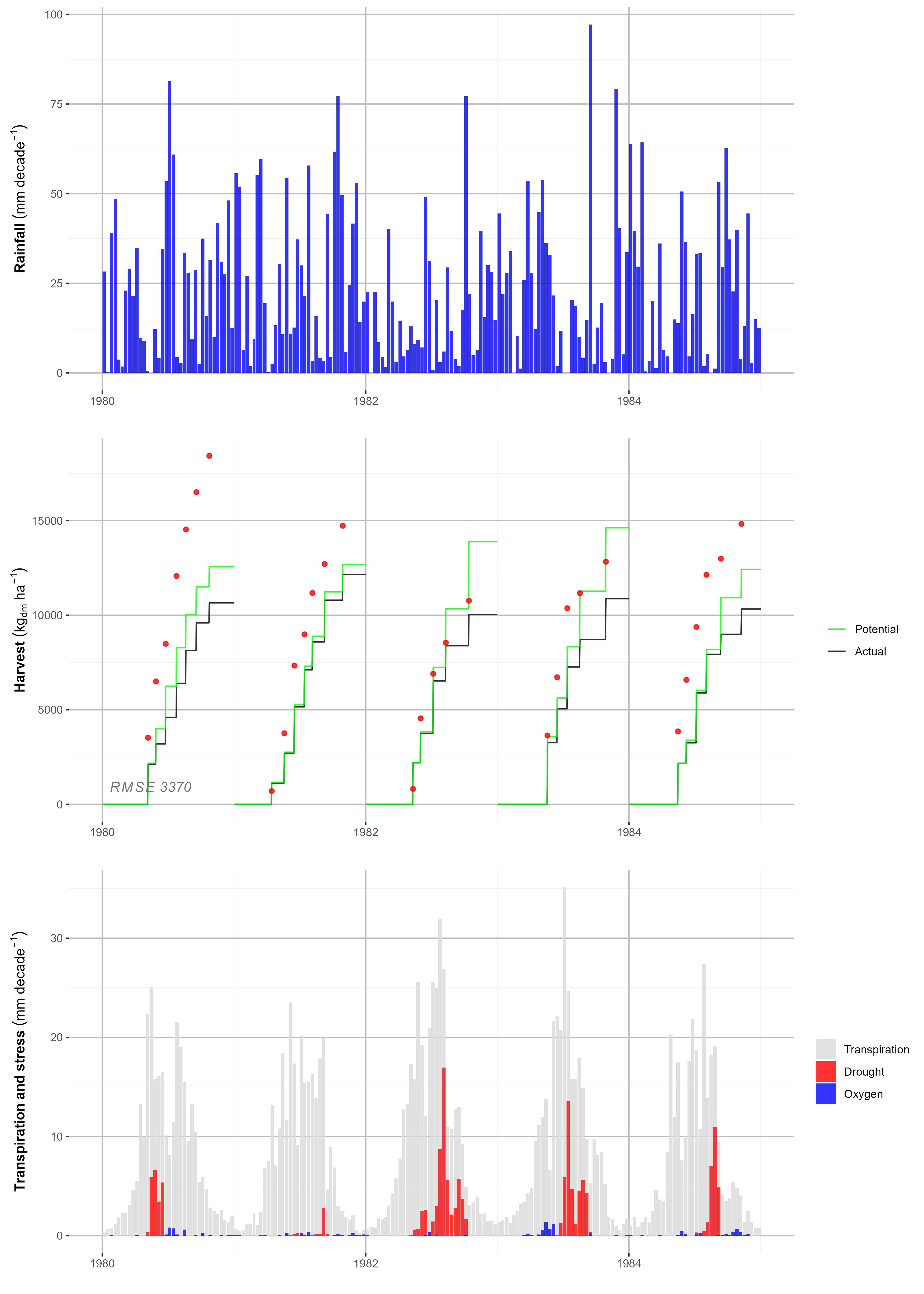
After running the SWAP simulation with the batch file (run_swap.cmd), the simulated yields can be visualized using SWAPtools via plot_swap.cmd. The layout and settings of the figure are defined in control_plot.inp. The example provided produces a figure with three panels:, rainfall; observed, potential and actual yields; and the actual transpiration along with reductions due to drought and oxygen stress. The resulting figure should resemble Figure 12.4.
Macropore flow
This case describes a field experiment where macropore flow is evident; a detailed description of the field experiment has been given by Smelt et al. (2003).
The precipitation excess is discharged from a field with a shallow groundwater level between 0.5 and 1.5 meter below the soil surface. Discharge occurs towards drains was simulated in the framework of pesticide leaching studies (Tiktak, Hendriks, and Boesten 2012) who also applied the same model tools at a national level (Tiktak et al. 2012).
**********************************************************************************
* Part 7: Preferential flow due to macropores

* Switch for macropore flow [0..1, I]:
  SWMACRO = 1                ! 0 = No macropore flow
                             ! 1 = Macropore flow

* If SWMACRO=1, specify:
* Switch for type of main bypass flow:
  SWMBF = 1                  ! 1 = Instantaneous bypass
                             ! 2 = Kinematic wave

* Switch for type of absorption [1..2, I]:
  SWABS = 1                  ! 1 = Sorptivity
                             ! 2 = Diffusion

* Switch for type of seepage [1..2, I]:
  SWSEP = 1                  ! 1 = Ernst
                             ! 2 = Youngs

* Macropore geometry variables:
  Z_ST = -220.0              ! Depth bottom static macropores [-1000..0 cm, R]
  Z_IC = -100.0              ! Depth bottom internal catchment domain [-1000..0 cm, R]
  VLMPSTSS = 0.04            ! Volume fraction of static macropores at soil surface [0..0.5 cm3/cm3, R]
  NUMSBDM = 4                ! Number of subdomains in internal catchment domain [0..20 -, I]
  DIPOMI = 10.0              ! Minimal diameter soil polygons (shallow) [0.1..1000 cm, R]
  DIPOMA = 50.0              ! Maximal diameter soil polygons (deep) [0.1..1000 cm, R]
  ZDIPOMA = 0.0              ! Depth below which soil polygons reach their maximum diameter  [-1000..0 cm, R]
                             ! (only required and used if VLMPSTSS = 0.0 and PPICSS = 0.0)
  ZNCRAR = -5.0              ! Depth at which dynamic crack area of soil surface is calculated
                             ! (only used if soil above depth ZNCRAR is not rigid) [-100..0 cm, R]

* Macropore geometry variables (optional):
  Z_TP = 0.0                 ! Depth top macropores for cover layer (default = 0.0) [-1000..0 cm, R]
  Z_MB50 = -160.0            ! Depth at which the static main bypass domain volume is half that at the top (default = (Z_IC+Z_ST)/2) [-1000..0 cm, R]

* If NUMSBDM>0, specifiy internal catchment geometry variables:
  PPICSS = 0.5               ! Proportion of internal catchment domain at soil surface [0..0.99 -, R]

* Internal catchment geometry variables (optional):
  Z_AH = -26.0               ! Depth bottom A-horizon (default = bottom first node) [-1000..0 cm, R]
  RZAH = 0.0                 ! Fraction macropores ended at bottom A-horizon (optional; default 0.0) [0..1 -, R]
  POWM = 1.0                 ! Power M for freq. distr. curve internal catchment domain (optional; default 1.0) [0..100 -, R]
  SPOINT = 1.0               ! Symmetry point for freq. distr. curve (optional; default 1.0) [0..1 -, R]
  SWPOWM = 0                 ! Switch for double convex/concave freq. distr. curve (optional, Y=1, N=0; default: 0) [0..1 -, I]

* Macropore hydrological variables:
  PNDMXMP = 0.0              ! Threshold value for ponding on soil surface before overland flow into macropores starts [0..10 cm, R]
  SHAPEFACMP = 1.5           ! Shape factor for description of macropore water exchange with matrix (theoretically between 1 and 2) [0..100 -, R]
  CRITUNDSATVOL = 0.1        ! Critical value for undersaturation volume [0..10 cm, R]

* Switch for eliminating Darcy flow unsaturated zone (absorption):
  SWDARCY = 1                ! 0 = Eliminate Darcy flow
                             ! 1 = Do not eliminate Darcy flow

* Switch for rapid drainage to drainage system (at least one drainage level needs to be specified) [0..1 -, I]:
  SWDRRAP = 1                ! 0 = no rapid drainage
                             ! 1 = rapid drainage

* If SWDRRAP=1, specify rapid drainage parameters:
 RAPDRARESREF = 50.0         ! Reference rapid drainage resistance [0..1.E+10 /d, R]
 RAPDRAREAEXP = 1.0          ! Exponent for reaction rapid drainage to dynamic crack width [0..100 -, R]
 NUMLEVRAPDRA = 1            ! Number of drainage system connected to rapid drainage [1..5, -, I]

* If SWDRRAP=1, specify shrinkage characteristics:
* SWSOILSHR = Switch for kind of soil for determining shrinkage curve: 0 = rigid soil, 1 = clay, 2 peat [0..2 -, I]
* SWSHRINP = Switch for determining shrinkage curve [1..2 -, I]:
*        1 = parameters for curve are given;
*        2 = typical points of curve are given
* GEOMFAC = Geometry factor (3.0 = isotropic shrinkage), [0..100, R]
*
* SHRPAR A to E = parameters for describing shrinkage curves,
* depending on combination of SWSOILSHR and SWSHRINP [-1000..1000, R]:
* SWSOILSHR = 0: 0 variables required (all dummies)
* SWSOILSHR = 1 and SWSHRINP 1: 3 variables required (SHRPAR A to C) (rest dummies)
* SWSOILSHR = 1 and SWSHRINP 2: 2 variables required (SHRPAR A to B) (rest dummies)
* SWSOILSHR = 2 and SWSHRINP 1: 5 variables required (SHRPAR A to E)
* SWSOILSHR = 2 and SWSHRINP 2: 4 variables required (SHRPAR A to D) (rest dummies)

 SWSOILSHR SWSHRINP THETCRMP GEOMFAC SHRPARA SHRPARB SHRPARC SHRPARD SHRPARE
         1        2    0.385     3.0   0.343  0.5390     0.0     0.0     0.0
         1        2    0.385     3.0   0.343  0.5392     0.0     0.0     0.0
         1        2    0.354     3.0   0.415  0.6350     0.0     0.0     0.0
         1        2    0.375     3.0   0.400  0.6400     0.0     0.0     0.0
         1        2    0.422     3.0   0.412  0.7840     0.0     0.0     0.0
         1        2    0.420     3.0   0.406  0.6883     0.0     0.0     0.0
         1        2    0.499     3.0   0.495  0.9000     0.0     0.0     0.0
         1        2    0.499     3.0   0.495  0.9000     0.0     0.0     0.0
* End of table

* Sorptivity characteristics:
* SWSORP = Switch for kind of sorptivity function [1..2 -, I]:
*      1 = Calculated from hydraulic functions according to Parlange (requires SORPFACPARL, rest dummies)
*      2 = Emperical function from measurements (requires SORPMAX, SORPALFA, rest dummies)
* SORPFACPARL = Factor for modifying Parlange function (optional; default 1.0) [0..100 -, R]
* SORPMAX = Maximal sorptivity at theta residual [0..100 cm/d**0.5, R]
* SORPALFA = Fitting parameter for emperical sorptivity curve [-10..10 -, R]

 SWSORP SORPFACPARL SORPMAX SORPALFA
      1        0.33     0.3      0.5
      1        0.33     0.3      0.5
      1        0.33     0.6      0.5
      1        0.50     5.0      0.5
      1        0.50     5.0      0.5
      1        0.50     5.0      0.5
      1        0.50     5.0      0.5
      1        0.50     5.0      0.5
* End of table

**********************************************************************************```
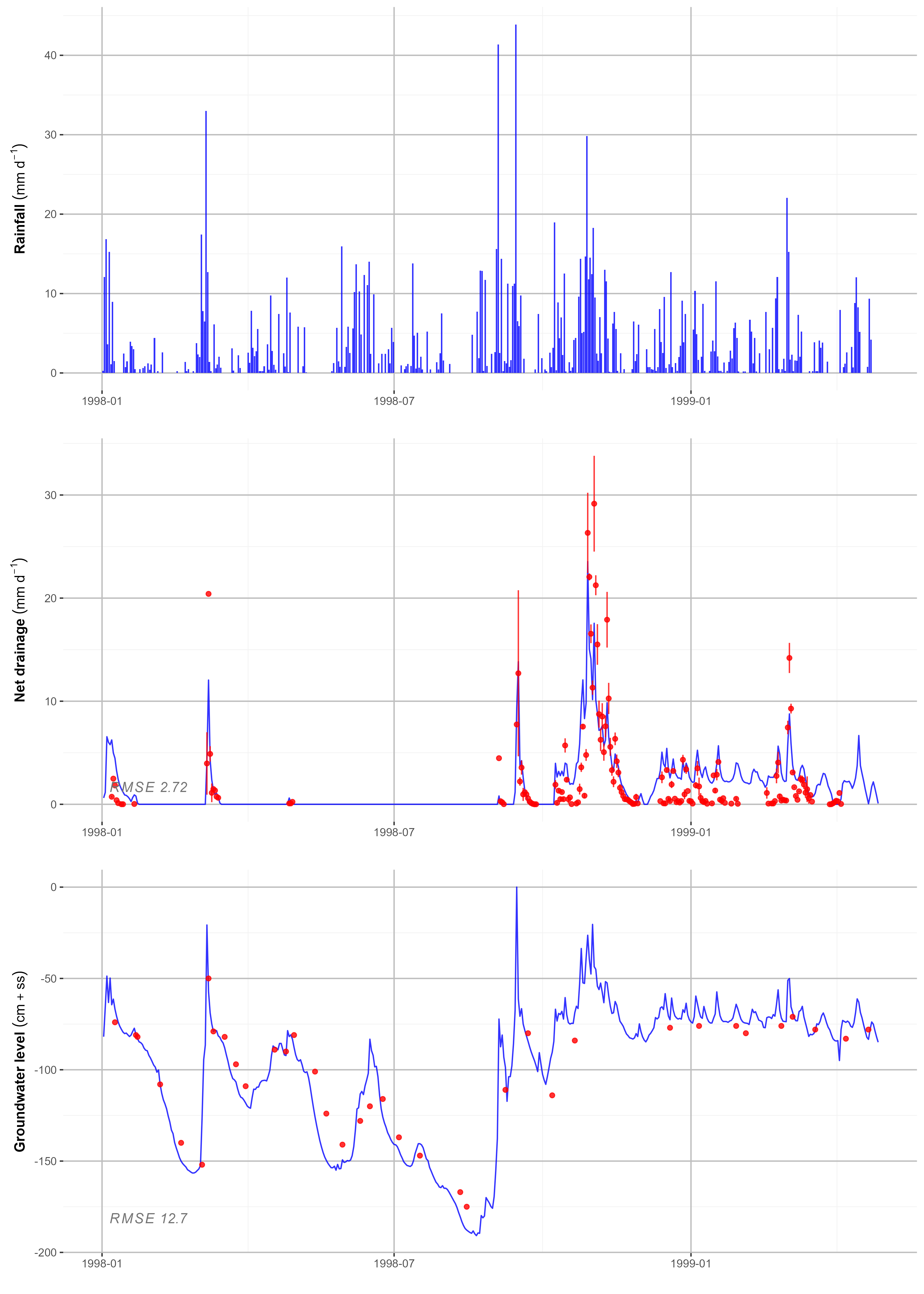
The model results can be visualized using SWAPtools via plot_swap.cmd. The example provided produces a figure with three panels:, rainfall; observed and simulated drainage discharge; and the observed and simulated groundwater level. The resulting figure should resemble Figure 12.5.
Salinity stress
Salinization is one of the major threats to agriculture worldwide, and is an increasing problem. In the Netherlands it is expected that salinization of arable land will increase up to 125.000 hectares (De Kempenaer, Brandenburg, and Hoof 2007).
Since 2012 field trials have been performed at the open-air laboratory of Salt Farm Texel in the Netherlands in order to investigate salt tolerance of different crops ( saltfarmtexel.com). Between 2012 and 2015 varieties of potatoes were daily irrigated (drip irrigation) with seven different salt concentrations located in 56 fields (maximum of eight replicas for each salt concentration). During the experiment, soil moisture of the top layer, soil water salinity at different depths and the crop yields were monitored (De Vos et al. 2016).
Meteorological data are gained from a nearby automatic Dutch national weather station De Kooy (KNMI). Potato growth parameters are based on standard potatoes for this region (Solanum Tuberosum; Fontane). A management factor was set to 0.80. For this example, simulation results are presented for three treatments with salinity concentrations 1.05, 2.29 and 4.99 mg cm-3 (corresponding to 4, 8 and 16 dS m-1, respectively). The threshold of soil water salt concentration above which root water uptake begins to decline was set at 0.732 mg cm-3, and the rate of decline beyond this threshold was defined as 0.0868 cm3 mg-1. Tip 12.8 illustrates the salt stress parameters, which is included in the *.crp input file.
**********************************************************************************
* Part 3: Salinity stress

* Switch salinity stress
  SWSALINITY = 1             ! 0 = No salinity stress
                             ! 1 = Maas and Hoffman reduction function

* If SWSALINITY=1, specify threshold and slope of Maas and Hoffman
  SALTMAX = 0.732            ! Threshold salt concentration in soil water  [0..100 mg/cm3, R]
  SALTSLOPE = 0.0868         ! Decline of root water uptake above threshold [0..1.0 cm3/mg, R]

**********************************************************************************
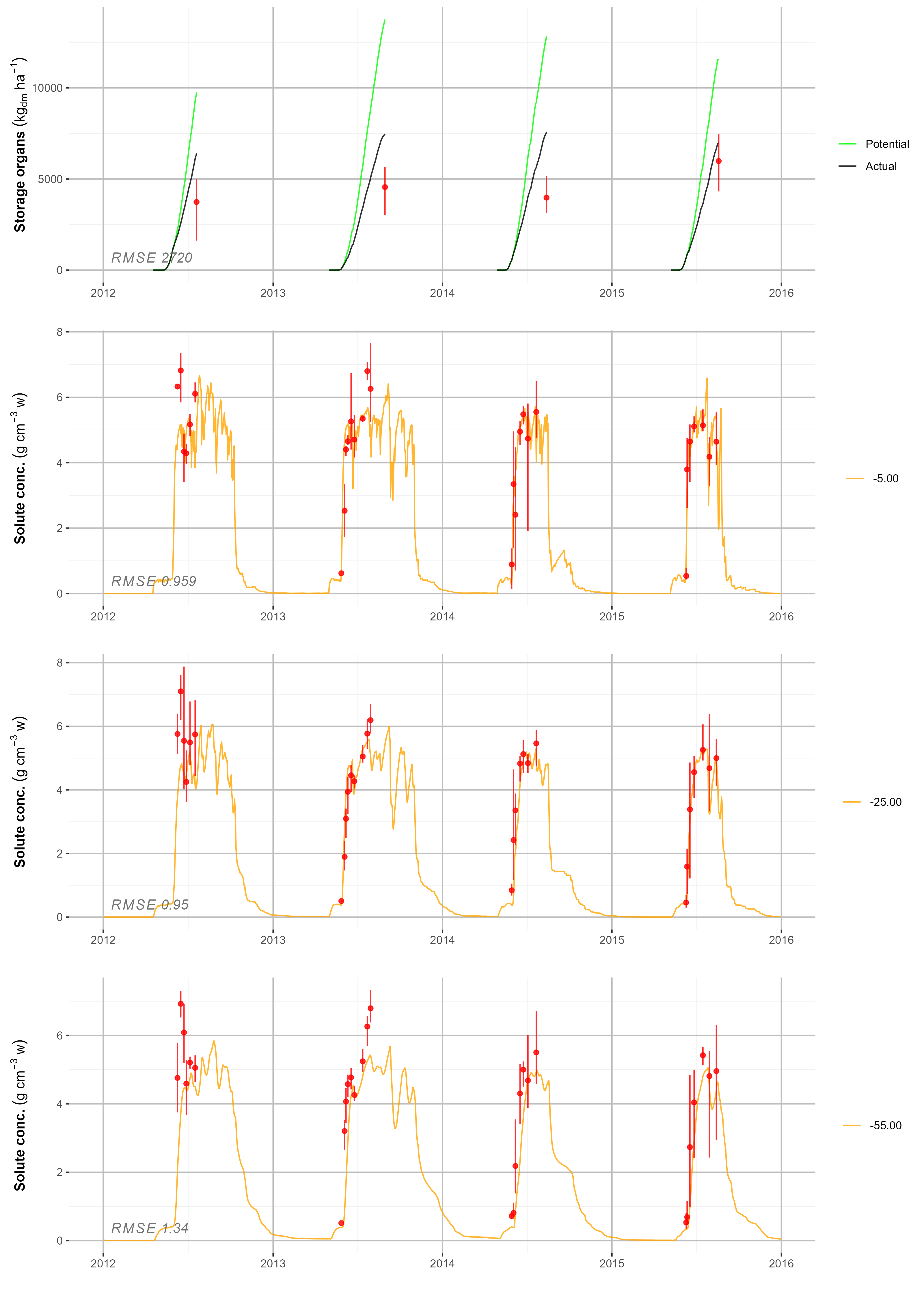
In this example, the R-package SWAPtools is used to perform multiple SWAP simulations. For each treatment, a simulation is run with different salinity concentrations of the irrigation water, provided in an Excel file. The batch file run_swap.cmd calls the R script run_swap.R with the argument control.inp. The procedure consist of three steps: pre-processing (converting the Excel to an SQLite database), the main process (executing SWAP), and post processing (visualizing the model results). Figure 12.6 presents the simulated yields and soil water salinity at three depth intervals for treatment with 16 dS m-1 (run 3).
Bierkens, M. F. P., and C. E. Puente. 1990.
“Analytically Derived Runoff Models Based on Rainfall Point Processes.” Journal Article.
Water Resources Research 26 (11): 2653–59.
https://doi.org/10.1029/WR026i011p02653.
Brauer, C. C. 2014. Modelling Rainfall-Runoff Processes in Lowland Catchments. PhD Thesis. Book. Wageningen University, The Netherlands.
De Kempenaer, J. G., W. A. Brandenburg, and L. J. W. van Hoof. 2007.
Het Zout En de Pap. Een Verkenning Bij Marktexperts Naar Lange Termijnmogelijkheden Voor Zilte Landbouw. Rapport Project “Markttrends Zilte Productie". Book. InnovatieNetwerk, Utrecht, The Netherlands.
http://edepot.wur.nl/25020.
De Vos, A., B. Bruning, G. van Straten, R. Oosterbaan, J. Rozema, and P. van Bodegom. 2016.
Crop Salt Tolerance Under Controlled Field Conditions in the Netherlands, Based on Trials Conducted at Salt Farm Texel. Book. SaltFarm Texel. Texel. The Netherlands.
www.saltfarmtexel.com as http://www.saltfarmtexel.com/application/files/5714/8776/5471/saltfarm-texel_brochure_A4.pdf.
Heinen, M., G. Bakker, and J. H. M. Wösten. 2020.
Waterretentie- En Doorlatendheidskarakteristieken van Boven- En Ondergronden in Nederland: De Staringreeks. Update 2018. Report 2987. Book. Wageningen Environmental Research, Wageningen.
https://doi.org/10.18174/512761.
Hopmans, J. W., and J. N. M. Stricker. 1989.
“Stochastic Analysis of Soil Water Regime in a Watershed.” Journal Article.
Journal of Hydrology 105 (1-2): 57–84.
https://doi.org/10.1016/0022-1694(89)90096-6.
Kroes, J. G., and I. Supit. 2011.
“Impact Analysis of Drought, Water Excess and Salinity on Grass Production in the Netherlands Using Historical and Future Climate Data.” Journal Article.
Agriculture Ecosystems and Environment 144: 370–81.
https://doi.org/10.1016/j.agee.2011.09.008.
Rozemeijer, J. C., Y. van der Velde, F. C. van Geer, G. H. de Rooij, P. J. J. F. Torfs, and H. P. Broers. 2010.
“Improving Load Estimates for NO3 and p in Surface Waters by Characterizing the Concentration Response to Rainfall Events.” Journal Article.
Environmental Science and Technology 44: 6305–12.
https://doi.org/10.1021/es101252e.
Smelt, J. H., R. F. A. Hendriks, L. J. T. van der Pas, A. M. Matser, A. van den Toorn, K. Oostindie, O. M. van Dijk-Hooijer, J. J. T. I. Boesten, and R. P. Scorza Junior. 2003. Transport of Water, Bromide Ion, Nutrients and the Pesticides Bentazone and Imidacloprid in a Cracking, Tile Drained Clay Soil at Andelst, the Netherlands, Alterra Rapport 289. Book. Alterra, Wageningen, The Netherlands.
Stricker, J. N. M., and W. Brutsaert. 1978.
“Actual Evapotranspiration over a Summer in the "Hupsel Catchment".” Journal Article.
Journal of Hydrology 39: 139–57.
https://doi.org/10.1016/0022-1694(78)90119-1.
Tiktak, A., R. F. A. Hendriks, and J. J. T. I. Boesten. 2012.
“Simulation of Movement of Pesticides Towards Drains with a Preferential Flow Version of PEARL.” Journal Article.
Pest Management Science 68: 290–302.
https://doi.org/10.1002/ps.2262.
Tiktak, A., R. F. A. Hendriks, J. J. T. I. Boesten, and A. M. A. van der Linden. 2012.
“A Spatially Distributed Model of Pesticide Movement in Dutch Macroporous Soils.” Journal Article.
Journal of Hydrology 470–471: 316–27.
https://doi.org/10.1016/j.jhydrol.2012.09.025.
Van den Eertwegh, G. A. P. H. 2002. Water and Nutrient Budgets at Field and Regional Scale: Travel Times of Drainage Water and Nutrient Loads to Surface Water. PhD Thesis. Book. Wageningen University, Wageningen, The Netherlands.
Van der Velde, Y., P. J. J. F. Torfs, S. E. A. T. M. van der Zee, and R. Uijlenhoet. 2012.
“Quantifying Catchment-Scale Mixing and Its Effect on Time Varying Travel Time Distributions.” Journal Article.
Water Resources Research 48: W06536.
https://doi.org/10.1029/2011WR011310.