10 Snow and frost
SWAP contains separate switches for simulating snow and frost conditions. When both switches are turned off, in the simulations precipitation and soil water remain unfrozen at temperatures below zero \(^\circ\)C. Snow is described in Section 10.1 and frost in Section 10.2.
10.1 Snow
When the snow option is switched on, SWAP simulates snowfall, accumulation of snow in a snowpack, and the water balance of the snowpack. The present approach is quite simple and consists of the most basic processes, including the insulating effect of snow on energy transport. Simulation of snowfall and the water balance of the snowpack is performed on a daily basis. Snowfall and snowpack are described in the next two sections.
10.1.1 Snowfall
Snowfall occurs when air temperature drops below a threshold value. In that case, precipitation falls partly or completely as snow. The division of total precipitation \(P\) (cm d-1) into snow \(P_s\) (cm d-1) and rain \(P_r\) (cm d-1) depends on the daily average air temperature. For air temperatures \(T_\text{av}\) (\(^\circ\)C) below the threshold temperature \(T_\text{snow}\) (\(^\circ\)C) all precipitation is snow, while for air temperatures above the threshold temperature \(T_\text{rain}\) (\(^\circ\)C) all precipitation is rain. Between both threshold temperatures, the snow fraction \(f_\text{snow}\) (-) and rain fraction \(f_\text{rain}\) (-) of the precipitation are obtained by linear interpolation:
\[ f_\text{snow} = \begin{cases} 1 & \text{for} \space T_\text{av} \leq T_\text{snow} \\ \frac{T_\text{rain} - T_\text{av}}{T_\text{rain} - T_\text{snow}} & \text{for} \space T_\text{snow} < T_\text{av} < T_\text{rain} \\ 0 & \text{for} \space T_\text{av} \geq T_\text{rain} \end{cases} \tag{10.1}\]
\[ f_\text{rain} = 1 - f_\text{snow} \tag{10.2}\]
\[ P_s = f_\text{snow} P \quad \text{and} \quad P_r = f_\text{rain} P \tag{10.3}\]
10.1.2 Snowpack
Snow that falls on the soil surface is accumulated in a snowpack, provided that the soil surface temperature is below 0.5 \(^\circ\)C. The water balance of the snowpack includes storage, the incoming fluxes snow and rain, and the outgoing fluxes melt and sublimation (Figure 10.1) and reads:
\[ S_\text{snow}^t - S_\text{snow}^{t-1} = (P_r + P_s - q_\text{melt} - q_\text{melt,r} - E_s) \Delta t \tag{10.4}\]
in which \(S_\text{snow}\) is snow storage at day \(t\) or the previous day \(t-1\) in cm water equivalent (cm w.e.), \(P_s\) and \(P_r\) are the two precipitation terms (cm w.e. d-1), \(q_\text{melt}\) and \(q_\text{melt,r}\) are two snow melt terms (cm w.e. d-1), \(E_s\) is snow sublimation (cm w.e. d-1), and \(\Delta t\) is the time step of one day.
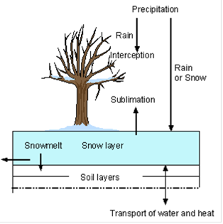
Two forms of snowmelt are included in the model:
Air temperature rise above a threshold value, according to the ‘degree-day model’ (Kustas, Rango, and Uijlenhoet 1994): \[ q_\text{melt} = \begin{cases} a(T_\text{av} - T_b) & \text{for} \space T_\text{av} > T_b\\ 0 & \text{for} \space T_\text{av} \leq T_b \end{cases} \tag{10.5}\] where \(a\) is the ‘degree-day factor’ (cm \(^\circ\)C-1 d-1), \(T_\text{av}\) is the daily average air temperature (\(^\circ\)C), and \(T_b\) is the base temperature (\(^\circ\)C) which is set to 0 \(^\circ\)C according to Kustas, Rango, and Uijlenhoet (1994). The value of \(a\) can be specified by the user and usually ranges between 0.35 and 0.60 cm \(^\circ\)C-1 d-1.
Heat release from rainfall \(P_r\) on the snowpack: additional melt will occur due to heat released by splashing raindrops. This snowmelt rate \(q_\text{melt,r}\) is calculated with (Fernández 1998; Singh et al. 1997): \[ q_\text{melt,r} = \begin{cases} \frac{P_r C_m T_\text{av}}{L_f} & \text{for} \space T_\text{av} > T_\text{snow}\\ 0 & \text{for} \space T_\text{av} \leq T_\text{snow} \end{cases} \tag{10.6}\] where \(C_m\) is the heat capacity of water (4180 J kg-1 \(^\circ\)C-1), \(L_f\) is the latent heat of fusion (333580 J kg-1), and \(T_\text{snow}\) is the temperature of the snowpack, which is set to 0 \(^\circ\)C.
The melt fluxes leave the snowpack as infiltration into the soil and/or runoff when the infiltration capacity of the soil is exceeded.
Snow can evaporate directly into the air, a process called sublimation. The sublimation rate \(E_s\) is taken equal to the potential evaporation rate \(E_p\) (see Chapter 3). When a snowpack exists, the evapotranspiration from the soil and vegetation is set to zero.
A snowpack on top of the soil surface has a large impact on soil temperatures. Because of the low thermal conductivity of snow (0.1-0.4 times the thermal conductivity of water), a snowpack can form a perfect insulating layer that will considerably dampen the effects of air temperature on soil temperature. The insulating effect of a snowpack on soil temperature is accounted for by calculating the temperature at the soil surface, the driving force for soil temperature calculations (see Chapter 9), taking into account the thermal conductivity and thickness of the snowpack. Therefore, the surface temperature \(T_\text{ss}\) (\(^\circ\)C) is calculated as a weighted average derived from the distances from the top of the snow cover and the first soil temperature node to the surface and the respective temperatures of air and soil, and thermal conductivities of snow and soil (Granberg et al. 1999):
\[ T_\text{ss} = \frac{T_1 + a T_\text{av}}{1 + a} \tag{10.7}\]
where:
\[ a = \frac{\lambda_\text{snow} \left(\frac{\Delta z_1}{2}\right)}{\lambda_1 \Delta z_\text{snow}} \tag{10.8}\]
with \(\lambda_1\) (J cm-1 \(^\circ\)C-1 d-1) and \(\Delta z_1\) (cm) are thermal conductivity and thickness of the first soil compartment. Thermal conductivity of the snowpack \(\lambda_\text{snow}\) (J cm-1 \(^\circ\)C-1 d-1) depends on the density \(\rho_\text{snow}\) (kg cm-3) of the snowpack (Granberg et al. 1999):
\[ \lambda_\text{snow} = k_\text{snow} \rho_\text{snow}^2 \tag{10.9}\]
where \(k_\text{snow}\) is a thermal conductivity parameter for snow (24.71∙108 J cm-5 kg-2 \(^\circ\)C-1 d-1). For \(\rho_\text{snow}\), the average value of 170∙10⁻⁶ kg cm-3 is taken (Granberg et al. 1999), so that \(\lambda_\text{snow}\) equals 71.4 J cm-1 \(^\circ\)C-1 d-1 (15% of \(\lambda_\text{water}\)).
Thickness of the snowpack \(\Delta z_\text{snow}\) (cm) is calculated from storage and density of snow, and the density of water (1000∙10-6 kg cm-3):
\[ \Delta z_\text{snow} = \frac{\rho_\text{water}}{\rho_\text{snow}} S_\text{snow} = \frac{1000}{170} S_\text{snow} \tag{10.10}\]
10.2 Frost
If the option for frost is activated, SWAP simulates the freezing of soil water when soil temperature drops below a threshold value \(T_\text{frz}\) (\(^\circ\)C). Soil ice has a significant impact on water flow and storage in the soil. To simulate this impact in situations where soil ice occurs, some transport parameters are adjusted. This is achieved by using a factor \(f_T(z)\), which introduces a correction when soil temperatures are below \(T_\text{frz}\) at depth \(z\). This correction factor is assumed to be linearly related to the fraction of soil ice \(f_\text{ice}(z)\) (-) at depth \(z\):
\[ f_T(z) = 1 - f_\text{ice}(z) \tag{10.11}\]
where \(f_\text{ice}(z)\) is the fraction of the free volumetric soil water content (actual water content minus residual water content) at depth \(z\).
According to measured data from Kujala (1991), \(f_\text{ice}(z)\) can reasonably well be described by a linear function of soil temperature \(T(z)\) (\(^\circ\)C) between two threshold temperatures:
\[ f_\text{ice}(z) = \begin{cases} 0 & \text{for} \space T(z) \geq T_\text{frz}\\ \frac{T_\text{frz} - T(z)}{T_\text{frz} - T_\text{mlt}} & \text{for} \space T_\text{mlt} < T(z) < T_\text{frz}\\ 1 & \text{for} \space T(z) \leq T_\text{mlt} \end{cases} \tag{10.12}\]
where \(T_\text{frz}\) is the temperature below which soil water starts freezing, and \(T_\text{mlt}\) is the temperature above which soil ice starts melting and below which all soil water except \(\theta_\text{res}\) is frozen. A value of \(T_\text{frz} < 0\) \(^\circ\)C expresses freezing point depression. \(T_\text{frz}\) and \(T_\text{mlt}\) are model input with default values of 0 and -1 \(^\circ\)C.
The following parameters are adjusted in case of soil ice:
Hydraulic conductivity \(K\): \[ K^*(z) = f_T(z)(K(z) - K_{\min}) \tag{10.13}\] where \(K^*(z)\) is the adjusted hydraulic conductivity at depth \(z\) (cm d-1) and \(K_{\min}\) is a very small hydraulic conductivity (cm d-1). For \(K_{\min}\) a default value is taken of \(10^{-10}\) cm d-1;
Actual crop uptake is reduced as: \[ S_a(z) = \alpha_\text{rf} S_a(z) \quad \text{with} \quad \alpha_\text{rf} = 0 \quad \text{for} \quad T(z) < 0 \; \text{$^\circ$C} \tag{10.14}\] where \(\alpha_\text{rf}\) is a multiplication factor for soil temperatures (-);
Drainage fluxes of all drainage levels: \[ q_{\text{drain},i}(z) = f_T(z) q_{\text{drain},i}(z) \tag{10.15}\] where \(q_{\text{drain},i}(z)\) is the drainage flux at depth \(z\) from drainage level \(i\) (cm d-1);
Bottom flux: \[ q_\text{bot} = f_T(z) q_\text{bot} \tag{10.16}\] where \(q_\text{bot}\) is the flux across the bottom of the modeled soil profile and \(z\) the bottom depth;
Boundary fluxes (drainage and bottom) when the available air volume is very low:
When drainage does not occur and the available air volume is very low (<0.01 cm cm-3), the bottom flux is reduced to zero.
When drainage occurs and the available air volume is very low (<0.01 cm cm-3), the drainage fluxes of frozen soil compartments above the drainage level are reduced to zero.
The (available) air volume in the soil \(V_\text{air}\) (cm) for a soil profile that becomes saturated equals: \[ V_\text{air} = \sum_{i=n}^m (\theta_{s,i} - \theta_i) \Delta z_i \tag{10.17}\] where \(\theta_{s,i}\) is the saturated water content (cm cm-3), \(\theta_i\) is the actual water content (cm³ cm-3), \(i\) is a particular node number, \(n\) is the node number of the bottom compartment, \(m\) is the node number of the highest soil compartment with a temperature below \(T_\text{mlt}\) starting to count from the bottom compartment, and \(\Delta z_i\) is the nodal distance \((z_i - z_{i+1})\).
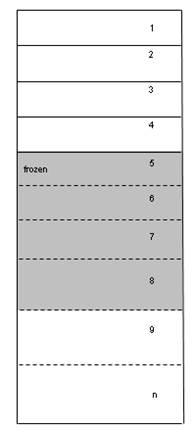
When a soil compartment is frozen (\(T(z) < T_\text{mlt}\)), the pore volume of the total soil profile becomes smaller, because only the compartments below this layer are used in the calculation.
An example is a soil in spring that is melting (Figure 10.2). The lower compartments were never frozen and the melting starts at the soil surface. It is possible that the first 4 compartments have melted and only the compartments 5 - 8 are frozen. Now the air volume is only calculated for compartments \(n\) (bottom) to \(m = 5\) (frozen). The following is then valid:
- When drainage does not occur and the available air volume is very low (<0.01 cm cm-3), the bottom flux is reduced to zero.
- When drainage does occur and the available air volume is very low (<0.01 cm cm-3), the drainage fluxes of all drainage systems that have a drainage level above the lowest frozen soil compartment are reduced to zero.
10.3 User instructions
Obviously, the options for snow and frost can only be used when the soil temperature simulation is activated.
For the snow option, the two threshold temperatures \(T_\text{rain}\) and \(T_\text{snow}\), the initial storage of snow at the beginning of the simulations \(S_\text{snow}\), and the ‘degree-day factor’ \(a\) are required as model input (Tip 10.1).
The frost option requires input for the two threshold temperatures \(T_\text{frz}\) and \(T_\text{mlt}\) (Tip 10.1).