| φsur,tar (cm) | φavg,max (cm) | hmax (cm) | Vuns,min (cm) |
|---|---|---|---|
| -180 | 0 | 0 | 0.0 |
| -160 | -80 | -100 | 1.5 |
| -140 | -90 | -150 | 2.0 |
| -120 | -100 | -200 | 2.5 |
| -100 | -120 | -250 | 3.0 |
| -80 | -130 | -300 | 4.0 |
5 Surface water management
5.1 Surface water balance
Surface water management options have been implemented in the SWAP model by taking account of the water balance of the surface water. The groundwater-surface water system is described at the scale of a horizontal subregion. The subregion has a single representative groundwater level and it is assumed that the soil profile occupies the whole surface area. This results in water balance terms of the soil profile that are computed per unit area (cm3 cm-2) and have the same numerical value for the sub-region as a whole. The surface water system is simplified to a control unit for which the following surface water balance equation is formulated:
\[ \frac{dV_\text{sur}}{dt} = q_\text{sup} - q_\text{dis} + q_\text{drain} + q_\text{crackfl} + q_\text{runoff} \tag{5.1}\]
where \(V_\text{sur}\) is the regional surface water storage (cm3 cm-2), \(q_\text{sup}\) is external supply to the control unit (cm3 cm-2 d-1), \(q_\text{dis}\) is discharge from control unit (cm3 cm-2 d-1), \(q_\text{drain}\) is regional drainage flow (cm3 cm-2 d-1), \(q_\text{crackfl}\) is bypass flow through cracks of a clay soil to drains or ditches (cm3 cm-2 d-1), and \(q_\text{runoff}\) is either surface runoff or surface runon (cm3 cm-2 d-1).
The regional surface water storage \(V_\text{sur}\) (cm3 cm-2) is the sum of the surface water storage in each order of the surface water system:
\[ V_{\text{sur}} = \frac{1}{A_{\text{reg}}} \sum_{i=1}^n L_i A_{\text{d},i} \tag{5.2}\]
in which \(A_\text{reg}\) is the total area of the sub-region (cm2), \(L_i\) the total length of channels/drains of order i in the sub-region (cm), and \(A_{\text{d},i}\) is the wetted area of a channel vertical cross-section (cm2). The wetted area \(A_{\text{d},i}\) is calculated from the surface water level \(\phi_\text{sur}\), the channel bed level, the bottom width, and the side-slope. Substitution of Equation 4.23 in Equation 5.2 yields the expression:
\[ V_\text{sur} = \sum_{i=1}^n \frac{A_{\text{d},i}}{L_i} \tag{5.3}\]
Channels of order \(i\) only contribute to the storage if \(\phi_\text{sur} > z_{\text{bed},i}\). The storage in tile drains is neglected. SWAP calculates the net discharge \(q_\text{dis} - q_\text{sup}\) for a given timestep and for specified surface water levels \(\phi_\text{sur}^j\) and \(\phi_\text{sur}^{j+1}\):
\[ q_\text{dis} - q_\text{sup} = \frac{V_\text{sur}^j (\phi_\text{sur}^j) - V_\text{sur}^{j+1} (\phi_\text{sur}^{j+1})}{\Delta t^j} + q_\text{drain} + q_\text{crackfl} + q_\text{runoff} \tag{5.4}\]
If the sum of the terms on the right hand side is positive, discharge has taken place and the supply is equal to zero. If the sum is negative, supply has taken place and the discharge is equal to zero.
The drainage flux is calculated by:
\[ q_\text{drain} = \sum_{i=1}^n \frac{\phi_\text{avg} - \phi_{\text{drain},i}}{\gamma_{\text{drain},i}} \tag{5.5}\]
where the drainage level \(\phi_{\text{drain},i}\) is in this case equal to the channel bed level, \(z_{\text{bed},i}\). When the groundwater level is situated above the highest bed level and with the surface water level is below the lowest one the total drainage flux. If the surface water level tends to rise to levels higher than the channel bed level \(z_{\text{bed},i}\), the latter is replaced by the surface water level.
Calculation of the discharge rate \(q_\text{dis}\) is the last step in solving Equation 5.4:
If the supply rate \(q_{\text{sup}}\) takes a positive value, the discharge is set to zero. The calculation of the supply rate is based on the comparison the target level and that actual surface water level. After establishing a target level it is examined whether the surface water level can take the target value. If necessary, surface water supply is used to attain the target level. The water supply should meet to the following criteria:
- The supply rate should not exceed a user defined value of the maximum supply rate \(q_\text{sup,max}\)
- Water supply only occurs when the surface water level takes a value below the water supply level. This water supply level is defined as a tolerance value in relation to the target level.
For the fixed weir, the discharge follows from the iterative procedure to establish a target level from the stage – discharge relationship. This relationship can either be expressed in tabulated form or as a power function for “weir flow” (see Section 5.1.2.1).
For a soil moisture controlled weir, the discharge follows simply from the water balance equation as given by Equation 5.4, with \(q_\text{sup}\) set to zero and the storage \(V_\text{sur}^{j+1}\) set equal to the storage for the target level. The discharge \(q_\text{dis}\) is then the only unknown left, and can be solved directly.
5.1.1 Multi-level drainage with imposed surface water levels
SWAP comprises an option for imposing a surface water level time series to be used as drainage level time series. When using this option it is assumed that the surface water level is equal for all drainage systems. Surface waters associated to the different drainage systems have open connections to each other and conduit resistances are neglected. This results in only one overall surface water level. The number of drainage systems to account for depends on the position of the groundwater level and the surface water level relative to the channel bed level.
5.1.2 Multi-level drainage with simulated surface water levels
Another option in the SWAP model is to simulate the surface water level on the basis of the control unit surface water balance. Then, the discharge is governed by either a fixed weir or an automated weir. The user can specify different water management periods for which the settings of the weirs can be different. During each time step, SWAP determines in subsequent order:
- the target level;
- whether the target level is reached, and the amount of external supply that is needed (if any);
- the discharge that takes place (if any) and the surface water level at the end of the time step.
Two options for describing the functioning of a weir are available: 1) the target level of a fixed weir coincides with the crest level, which has a constant value within a certain management period, or 2) the target level of a soil moisture controlled weir is a function of a soil moisture state variable and is defined by a water management scheme.
5.1.2.1 Fixed weir
The fixed weir-option employs a power function based ‘stage-discharge’ relationship \(q_\text{dis}(\phi_\text{sur})\) for which the parameters in the input are specified in SI-units or a tabulated relationship. The power function based ‘stage-discharge’ relationship reads as:
\[ q_\text{dis} = \frac{Q_\text{dis}}{A_\text{cu}} = \frac{\alpha_\text{weir} (\phi_\text{sur} - z_\text{weir})^{\beta_\text{weir}}}{A_\text{cu}} \tag{5.6}\]
in which \(Q_\text{dis}\) is the volumetric discharge (m3 s-1), \(A_\text{cu}\) is the area of the control unit (m2), \(z_\text{weir}\) is the weir crest level (m), \(\alpha_\text{weir}\) is the discharge coefficient (m3-\(\beta\) d-1) and \(\beta_\text{weir}\) is the discharge exponent (-). For a broad-crested rectangular weir, \(\alpha_\text{weir}\) is (approximately) given by 1.7 times the width of the weir.
The stage-discharge relationship can optionally be specified by a table. In that case, the relationship should be defined for each management period.
5.1.2.2 Soil moisture controlled weir management
This model option assumes the target level of a weir to be controlled by one or more soil moisture state variables. The so-called water management scheme defines the setting of the water level \(\phi_\text{sur,tar}\) aimed for in relation to a soil moisture state variable. The target level is defined as a combinational function of three state variables related to soil moisture:
- the average groundwater level \(\phi_\text{avg}\) (cm). Lower target levels at higher groundwater levels may prevent waterlogging and can contribute to minimize crop yield reduction.
- the soil water pressure head \(h\) (cm) at a certain depth. A soil water pressure value appears to be a better indicator for water logging in nature reserves than a groundwater level criterion (Par.).
- the capacity of the unsaturated soil profile to store water \(V_\text{uns}\) (cm). This state variable is an indicator for the possibility of buffering extreme rainfall events. Maintaining a certain minimum amount of storage reduces the risk of flooding and subsequent discharge peaks.
During the simulation, the SWAP model selects the target level for which all three criteria are met. A scheme maintained by a soil moisture controlled weir is illustrated in Table 5.1. The minimum target level is specified in the first column. The second, third, and fourth column represent values for the corresponding groundwater level, soil water pressure head, and soil water storage capacity. The first row contains zeros, indicating that irrespective of the conditions, the minimum target level should never drop below that level.
To avoid the target level reacting too fast on the prevailing groundwater level, a maximum drop rate parameter has been introduced specifying the maximum permitted change of the target level per time unit (cm d-1). The limitation of the target level change can become effective in periods with surface water supply combined with a rising groundwater level.
In periods with heavy rainfall and high discharge, the maximum capacity of a soil moisture controlled weir can be reached and the crest level will drop to its minimum level. Then, the surface water level is not controlled by any of the criteria mentioned before any longer, but will be a function of the discharge characteristics of the surface water infrastructure. Therefore, the management scheme of a soil moisture controlled weir should always be combined with a table defining a stage discharge relationship. This tabulated relationship should be defined for every management period. The minimum level of management scheme should be identical to the minimum level of the discharge relationship.
5.2 User instructions
5.2.1 Input instructions
The user first has to select the option for extended drainage (Tip 5.1).
Parameters and input variables are specified in a separate file called drfil. The input data are given in 2 sections:
First, the user should specify the altitude of the control unit (soil surface), with respect to a certain reference level (altcu). In Section 2, water management levels are given with respect to the same reference. The user may choose to define the soil as surface reference level by specifying zero for the altitude. A flow chart of the input for the surface water module (section 2 in the input file) is given in Figure 5.1. The user should make selections for the kind of surface water system (swsrf) and the kind of control (swsec). The different parts of section 2 are described hereafter.
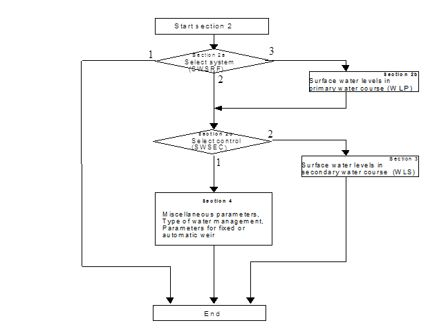
Section 2 starts with a switch (Section 2a, variable swsrf) for three options:
- No surface water system is simulated;
- Surface water system is simulated with no separate primary water course;
- Surface water system is simulated with a primary water course (level 1) separate from the control unit
If the first option (swsrf = 1) has been chosen, the user may skip the rest of Section 2. For the second or third option (swsrf = 2 or 3), the user has also to specify how the surface water level in the control unit is determined (section 2c, variable swsec):
- The surface water level is simulated;
- The surface water level is obtained from input data.
If the third option (swsrf = 3) has been chosen, the user should also specify (section 2b) the time variation of the surface water level in the primary water course. The specification is done in terms of data pairs (date, water level). To obtain levels at intermediate dates, the model performs a linear interpolation.
If the option is chosen to obtain surface water levels from input data (swsec = 1), the surface water level of the secondary watercourse has to be specified in the form of data pairs (section 3).
If the option is chosen to simulate surface water levels (swsec = 2), the user has to specify how the surface water system in the control unit functions and how it is managed (section 4).
Section 4 starts with some miscellaneous parameters (section 4a):
- the initial surface water level in the control unit;
- the criterion for detecting oscillation of the surface water level;
- the number of water management periods.
In the next section 4b, the management periods are defined as well as the type of water management: 1. fixed weir crest; 2. automatic weir, the water supply capacity and a tolerance value (wldip). The tolerance value wldip relates the water supply level to the target level preventing oscillations and too fast unrealistic responses of surface water management to the prevailing conditions. This tolerance can be seen as the allowed dip of the surface water level and can take a value of e.g., 10 cm. An appropriate setting of this parameter can save a substantial amount of water.
Dependent on the discharge relationship for the weir, the user has to specify:
- either Section 4c (swqhr=1, exponential relation)
- or section 4d (swqhr=2, relation given as table)
If an exponential relation is chosen, then for each water management period with a fixed weir crest using weir characteristics, the user should specify (section 4c):
Size of the control unit (catchment) (ha);
A table with weir characteristics for each management period:
- Index for management period (-);
- Elevation (H) of the weir crest (cm);
- Discharge coefficient α_input (m³-β s-1);
- Discharge exponent β (-).
Head-discharge relationships are given in SI-units, i.e., m for length and s for time and the discharge is computed as a volume rate (m3 s-1). To facilitate the input for the user, we conformed to hydraulic literature. This implies that the user has to specify the weir characteristics that define a relationship of the following form:
\[ Q = \alpha_\text{input} H^\beta \tag{5.7}\]
where \(Q\) is the discharge (m3 s-1), \(H\) is the head above the crest (m), and \(\alpha_\text{input}\) is a weir coefficient (m3-\(\beta\) s-1), \(\beta\) is a weir exponent (-). The preparatory work that the user has to do is to compute the value of \(\alpha_\text{input}\) from the various coefficients preceding the upstream head above the crest. For instance, for a broad-crested rectangular weir, \(\alpha_\text{input}\) is (approximately) given by:
\[ \alpha_\text{input} = 1.7b \tag{5.8}\]
where 1.7 is the discharge coefficient of the weir (based on SI-units), \(b\) is the width of the weir (m). To correct for units, SWAP carries out the following conversion:
\[ \alpha_\text{weir} = \frac{8.65 \times 100^{(1-\beta)}}{A_\text{cu}} \tag{5.9}\]
where \(A_\text{cu}\) is the size of the control unit (ha). The model requires input of the size of the control unit (\(A_\text{cu}\)), which in simple cases will be identical to the size of the simulation unit.
If the discharge relation is described using a table (swqhr = 2), then for each water management period with a fixed weir crest using weir characteristics, the user should specify a table in Section 4d.
In section 4e of the input file, the required parameters should be given to introduce an automatic weir (swman = 2) controlled by soil moisture characteristics (see also Section 5.1.2.2). For each management period with an automatic weir the user should specify in section 4e:
- the maximum allowed drop rate of the water level setting;
- the depth (hdepth) in the soil profile for a comparison between simulated and required soil moisture criterion (hcrit).
The three state variables (gwlcrit, hcrit, vcrit) that define the target weir level are given in a separate table.