| Par | SWAP | Unit | Range | Default | 4u | 5s | 6u | 7s | 8u | 9s | 10u | 11s |
|---|---|---|---|---|---|---|---|---|---|---|---|---|
| θr | ORES | m3 m-3 | [0,1] | 1 | 1 | 1 | 1 | 1 | 1 | 1 | 1 | |
| θs | OSAT | m3 m-3 | [0,1] | 1 | 1 | 1 | 1 | 1 | 1 | 1 | 1 | |
| α1 | ALFA | cm-1 | [10-4,100] | 1 | 1 | 1 | 1 | 1 | 1 | 1 | 1 | |
| n1 | NPAR | - | [1.001,9] | 1 | 1 | 1 | 1 | 1 | 1 | 1 | 1 | |
| λ | LEXP | - | [-25,25] | 1 | 1 | 1 | 1 | 1 | 1 | 1 | 1 | |
| Ks | KSATFIT | cm d-1 | [10-5,105] | 1 | 1 | 1 | 1 | 1 | 1 | 1 | 1 | |
| h0 | H0 | cm | [108,-105] | -106.8 | 0 | 1 | 0 | 1 | 1 | 1 | 1 | 1 |
| ha | HA | cm | [-105,0] | 1/α1 | 0 | 0 | 0 | 0 | 1 | 1 | 1 | 1 |
| α2 | ALFA_2 | cm-1 | [10-4,100] | 0 | 0 | 1 | 1 | 0 | 0 | 1 | 1 | |
| n2 | NPAR_2 | - | [1.001,9] | 0 | 0 | 1 | 1 | 0 | 0 | 1 | 1 | |
| w1 | OMEGA_1 | - | [10-4,0.9999] | 0 | 0 | 1 | 1 | 0 | 0 | 1 | 1 | |
| ωK | OMEGA_K | - | [10-8,0.1] | 0 | 0 | 0 | 0 | 1 | 1 | 1 | 1 | |
| a | APAR | - | [-5,0] | -1.5 | 0 | 0 | 0 | 0 | 1 | 1 | 1 | 1 |
2 Soil water flow
2.1 Basic equations
Gradients of the soil water potential cause soil water movement. Darcy’s equation is commonly used to quantify this soil water movement. For one-dimensional vertical flow, Darcy’s equation can be written as (Heinen et al. 2024):
\[ q=-K\left(h\right)\frac{\partial\left(h+z\right)}{\partial z} \tag{2.1}\]
where \(q\) is soil water flux density (positive upward) (cm3 cm-2 d-1 = cm d-1), \(K(h)\) is hydraulic conductivity (cm d-1), \(h\) is soil water pressure head (cm), and \(z\) is the vertical coordinate (cm), taken positively upward.
Water balance considerations of an infinitely small soil volume result in the continuity equation for soil water:
\[ \frac{\partial \theta}{\partial t}= -\frac{\partial q}{\partial z} -S_\text{a}\left(h\right) -S_\text{d}\left(h\right) -S_\text{m}\left(h\right)+ S_\text{si}\left(h\right) \tag{2.2}\]
where \(\theta\) is volumetric water content (cm3 cm-3), \(t\) is time (d), \(S_\text{a}\left(h\right)\) is soil water extraction rate by plant roots (cm3 cm-3 d-1), \(S_\text{d}\left(h\right)\) is the extraction rate by drain discharge in the saturated zone (cm3 cm-3 d-1), \(S_\text{m}\left(h\right)\) is the exchange rate with macro pores (cm3 cm-3 d-1), and \(S_\text{si}\left(h\right)\) is the subsurface irrigation rate (cm3 cm-3 d-1).
Combination of Equation 2.1 and Equation 2.2 provides the general water flow equation in variably saturated soils, known as the Richards equation:
\[ \frac{\partial \theta}{\partial t} = \frac{\partial \left[K\left(h\right) \left(\frac{\partial h}{\partial z} +1\right)\right]}{\partial z} -S_\text{a}\left(h\right) -S_\text{d}\left(h\right) - S_\text{m}\left(h\right)+ S_\text{si}\left(h\right) \tag{2.3}\]
SWAP applies Richards equation integrally for the unsaturated-saturated zone, including possible transient and perched groundwater levels. SWAP solves Equation 2.3 numerically, using specified boundary conditions and relations between \(\theta\), \(h\) and \(K\).
2.2 Soil hydraulic functions
2.2.1 General: Mualem - van Genuchten
SWAP uses the Mualem-Van Genuchten functions (Mualem 1976; Van Genuchten 1982) which have been used in numerous studies and form the base of several national and international data-bases (Carsel and Parrish 1988; Yates et al. 1992; Leij et al. 1996; Wösten et al. 2001; Vereecken et al. 2010). The analytical \(\theta\left(h\right)\) function proposed by Van Genuchten (1980) reads:
\[ \theta = \theta_\text{res}+\left(\theta_\text{sat} - \theta_\text{res} \right) \left(1+ \left| \alpha h\right|^n \right)^{-m} \tag{2.4}\]
where \(\theta_\text{sat}\) is the saturated water content (cm3 cm-3), \(\theta_\text{res}\) is the residual water content in the very dry range (cm3 cm-3) and \(\alpha\) (cm-1), \(n\) (-) and \(m\) (-) are empirical shape factors. Without loosing much flexibility, \(m\) can be taken equal to:
\[ m=1-\frac{1}{n} \tag{2.5}\]
Using the above \(\theta\left(h\right)\) relation, with \(m = 1-1/n\), and applying the theory on unsaturated hydraulic conductivity by Mualem (1976), the following \(K\left(q\right)\) function results:
\[ K = K_\text{sat} S^\lambda_\text{e} \left[ 1-\left( 1-S^{\frac{1}{m}}_\text{e}\right)^m\right]^2 \tag{2.6}\]
where \(K_\text{sat}\) is the saturated conductivity (cm d-1), \(\lambda\) is a shape parameter (-) depending on flow path tortuosity, and \(S_\text{e}\) is the relative degree of saturation defined as:
\[ S_e = \frac{\theta-\theta_\text{res}}{\theta_\text{sat}-\theta_\text{res}} \tag{2.7}\]
The numerical solution to the Richards equation requires an expression of the differential water capacity \(C\) (cm-1), which is defined as the derivative of \(\theta\) to \(h\) (Equation 2.4):
\[ C = \frac{\text{d} \theta}{\text{d} h} = \alpha m n \left| \alpha h\right|^{n-1} \left( \theta_\text{sat} - \theta_\text{res}\right) \left( 1 + \left| \alpha h\right|^n\right)^{-\left(m+1\right)} \tag{2.8}\]
A numerical approach to Equation 2.3 yielding a steady-state solution requires an implicit treatment of the hydraulic conductivity. This implies the use of the derivative of the hydraulic conductivity to the pressure head \(\text{d}K/\text{d}h\). Expressions are given in Appendix C.
A bi-modal version of the the Mualem-Van Genuchten functions is available as one of the models included in the Peters - Durner - Iden model as presented in Section 2.2.5.
According to Peters, Durner, and Wessolek (2011), the lower limit of \(\lambda\) is related to the \(m\) parameter which depends on the requirements of the \(K(h)\) relationship is: this should monotonous and concave. A monotonous and concave relationship results if \(\lambda > -2/m\) (monotonous only) or \(\lambda > 1 – 2/m\) (monotonous and concave) (if bi-modal then use the largest value of \(m_1\) and \(m_2\)). The check for monotonicity and concavity is performed at input.
2.2.2 Modification near saturation
Near saturation a modification to the Mualem-Van Genuchten function (Schaap and Van Genuchten 2006) has been implemented in SWAP. The modification is based on the introduction of a small minimum capillary height \(h_\text{e}\) which can be regarded as an air-entry value, causing a minor shift in the retention curve (Vogel, Genuchten, and Cislerova 2001). We follow Ippisch, Vogel, and Bastian (2006) by defining the relative water content as:
\[ S_\text{e}= \begin{cases} \frac {1} {S_\text{c}} \left [ 1+|\alpha h|^n \right ]^{-m} & h < h_\text{e} \\ 1 & h \ge h_\text{e} \end{cases} \tag{2.9}\]
where \(S_\text{c}\) is the relative saturation at the cut-off point \(h_\text{e}\) in the original Van Genuchten model, given by:
\[ S_\text{c} = \left[1+|\alpha h_\text{e}|^n\right]^{-m} \tag{2.10}\]
The hydraulic conductivity is then given by:
\[ K=\begin{cases} K_\text{sat}\left(S_\text{e}\right)^\lambda \left[\frac{1-\left( 1- \left( S_\text{e} S_\text{c}\right)^\frac{1}{m}\right)^m}{1-\left( 1- \left( S_\text{c}\right)^\frac{1}{m}\right)^m} \right]^2 & S_\text{e} < 1\\ K_\text{sat} & S_\text{e} \ge 1 \end{cases} \tag{2.11}\]
This model reduces to Equation 2.4 and Equation 2.6 for \(h_\text{e}\) = 0. For a detailed discussion of above equations we refer to Vogel, Genuchten, and Cislerova (2001), Schaap and Van Genuchten (2006) and Ippisch, Vogel, and Bastian (2006). They showed that this modification affects the shape of the retention curve only minimally relative to the original function. However, the impacts on the unsaturated hydraulic conductivity of fine-textured soils can be large.
To avoid numerical instabilities of the solution scheme, the soil moisture retention curve in the range -0.01 > \(h\) > 1.05 \(h_\text{e}\) cm is approached by a cubic spline of which the parameters preserve the continuity of the soil moisture retention curve and the differential moisture capacity function.
A second modification concerns the saturated hydraulic conductivity itself. The parameter \(K_\text{sat}\) of the \(K\left(S_\text{e}\right)\) relation is usually derived from experiments with unsaturated flow. These experiments may yield a poor estimate of the hydraulic conductivity at saturated conditions where soil structure usually dominates soil texture. However, to simulate accurately runoff conditions and drainage, a correct value of the saturated hydraulic conductivity is essential. Therefore SWAP users may specify in addition to the parameter \(K_\text{sat}\) the experimentally determined value of the saturated hydraulic conductivity \(K_\text{sat,exp}\). Close to saturation, in the range \(0 > h > -2\) cm, SWAP will linearly interpolate between \(K_\text{sat,exp}\) and \(K\left(S_\text{e}\right)\) at \(h = -2\) cm.
2.2.3 Soil hydraulic functions as tables
The (modified) uni-modal Mualem – van Genuchten representation of the \(\theta \left(h\right)\) and \(K\left( \theta\right)\) or \(K\left(h\right)\) relationships is just one of the many alternatives that are available in literature. Leij, Russell, and Lesch (1997) listed 14 such relationships commonly used in soil physics, Leong and Rahardjo (1997) presented eight relationships often used in geotechnical science, and Kosugi, Hopmans, and Dane (2002) described the most widely used expressions, including those of Brooks and Corey (1964, 1966) and Van Genuchten (1980). Currently in SWAP it has been decided not to implement many alternatives in the source code. Instead, the user is given the possibility to supply \(\theta \left(h\right)\) and \(K\left(h\right)\) relationships as tabulated input. In that way any relationship can be considered. During the computations interpolation is used to obtain \(\theta\), \(K\), \(C \left(= \mathrm{d}\theta/\mathrm{d}h\right)\) and \(\mathrm{d}K/\mathrm{d}h\) for any \(h\). Interpolation is done as piecewise cubic Hermite interpolation, preserving the monotonic character of the relationships (using PCHIP routines from the public domain software library SLATEC). Due to the interpolation method, the outcome does depend on the user-supplied information in the input tables. Best results are obtained when the \(h\)-\(\theta\)-\(K\) tables contain many data points nicely distributed over all variables, with special attention to data close to saturation and data close to wilting point and beyond. For example, in case the user has data available measured in the laboratory it is advised to first describe these data by some kind of analytical expression, and then derive tables based on this analytical expression. Experience has shown that supplying a coarse (or irregular) grid of \(h\)-\(\theta\)-\(K\) data points may cause unrealistic behaviour of the interpolated results, e.g. in the derivation of \(C\).
2.2.4 Hysteresis
Hysteresis refers to non-uniqueness of the \(\theta(h)\) relation and is caused by variations of the pore diameter (inkbottle effect), differences in radii of advancing and receding meniscus, entrapped air, thermal gradients and swelling/shrinking processes (Hillel 1980; Feddes et al. 1988). Gradual desorption of an initially saturated soil sample gives the main drying curve, while slow absorption of an initially dry sample results in the main wetting curve. In the field partly wetting and drying occurs in numerous cycles, resulting in so-called drying and wetting scanning curves lying between the main drying and the main wetting curves (Figure 2.1).
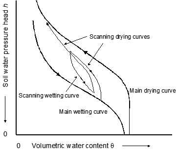
In simulation practice, often only the main drying curve is used to describe the \(\theta(h)\) relation. This is mainly due to the time and costs involved in measurement of the complete \(\theta(h)\) relationship, including the main wetting, the main drying and the scanning curves, especially in the dry range. For instance, a generally applied soil hydraulic data base in The Netherlands, known as the Staring series (Heinen, Bakker, and Wösten 2020; Heinen et al. 2022), contains only \(\theta(h)\) data of the main drying curve. Nevertheless, it is obvious that the simulation of infiltration events with the main drying curve can be inaccurate. Therefore the scaling method of Scott, Farquhar, and Kouwen (1983), who derived scanning curves by rescaling the main wetting or the main drying curve to the actual water content, has been implemented in SWAP.
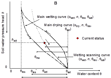
The main drying and main wetting curve are described analytically with the Mualem-van Genuchten parameters (\(\alpha\), \(n\), \(\theta_\text{res}\), \(\theta_\text{sat}\), \(K_\text{sat}\), and \(\lambda\)). Some of the parameters describing the main wetting and main drying curve are related. We assume \(\theta_\text{res}\) and \(\theta_\text{sat}\) to be equal for both curves. Usually the \(K(\theta)\) function shows only minor hysteresis effects, which can be achieved by choosing for the main wetting and main drying curve a common value for \(n\). Ultimately the two curves only differ in the parameter \(\alpha\), as depicted in Figure 2.2 (a) and Figure 2.2 (b). The scanning curves are derived by linear scaling of either the main wetting or main drying curve, such that the scanning curve approaches the main wetting curve in case of a wetting scanning curve and the main drying curve in case of a drying scanning curve.
The scaling principle in case of a drying scanning curve is depicted in Figure 2.2 (a). Based on its wetting and drying history, at a certain time and depth the soil shows an actual water content \(\theta_\text{act}\) at the soil water pressure head \(h_\text{act}\). The valid drying scanning curve should pass through the point (\(\theta_\text{act}\), \(h_\text{act}\)), and approach the main drying curve at smaller water contents, so that it will approach res when completely dried out. The same counts for the wetting scanning curves, these will all end up in \(\theta_{sat}\) when completely saturated.
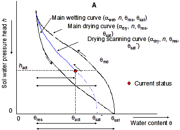
The drying scanning curves are derived in such a way that the combination of the actual pressure head \(h_\text{act}\) and the actual water content \(\theta_\text{act}\) are described by the parameters of the main drying curve with adjusted parameter \(\theta_\text{sat}\). We may define \(\theta_\text{md}\) as the water content of the main drying curve at \(h_\text{act}\), and \(\theta_\text{sat}\) as the saturated water content of the drying scanning curve. The main drying curve is linearly scaled with a factor \(f_\text{hyst}\) (Figure 2.2 (a)):
\[ f_\text{hyst} = \frac {\theta^*_\text{sat} - \theta_\text{res}} {\theta_\text{sat} - \theta_\text{res}} = \frac {\theta_\text{act} - \theta_\text{res}} {\theta_\text{md} - \theta_\text{res}} \tag{2.12}\]
from which it follows that
\[ \theta^*_\text{sat} = \theta_\text{res} + \left ( \theta_\text{sat} - \theta_\text{res}\right )f_\text{hyst} \tag{2.13}\]
The only unknown in Equation 2.12 and Equation 2.13 is \(\theta_\text{sat}^*\), which can be solved directly. In this case the parameter \(\theta_\text{res}\) of the main wetting curve is also scaled with the factor \(f_\text{hyst}\). The drying scanning curve is described accordingly with the parameters (\(\alpha_\text{dry}\), \(f_\text{hyst}\)). As long as the soil keeps drying, this drying scanning curve is valid.
The opposite occurs when the soil gets wetter. In this case the parameter \(\theta_\text{res}\) of the main wetting curve is also scaled with the factor \(f_\text{hyst}\). Again we start from the arbitrary actual water content \(\theta_\text{act}\) at the soil water pressure head \(h_\text{act}\), and now define \(\theta_\text{mw}\) as the water content of the main wetting curve at \(h_\text{act}\). The residual water content of the wetting scanning curve \(\theta^*_\text{res}\) is adapted according to (Figure 2.2 (b)):
\[ f_\text{hyst} = \frac {\theta_\text{sat} - \theta^*_\text{res}} {\theta_\text{sat} - \theta_\text{res}} = \frac {\theta_\text{sat} - \theta_\text{act}} {\theta_\text{sat} - \theta_\text{mw}} \tag{2.14}\]
from which it follows that
\[ \theta^*_\text{res} = \theta_\text{sat} - \left ( \theta_\text{sat} - \theta_\text{res}\right )f_\text{hyst} \tag{2.15}\]
From Equation 2.15 \(\theta_\text{res}^*\) can be directly solved. The wetting scanning curve is accordingly described with the parameters (\(\alpha_\text{wet}\), \(f_\text{hyst}\)), and is valid as long as the soil keeps wetting. The factor \(f_\text{hyst}\) has a value between 0 and 1. Due to stability reasons a minimum and maximum value are used, therefore \(f_\text{hyst}\) has a value between 0.1 and 0.9. As the wetting-drying history is different at each soil depth, each node may show a different scanning curve.
The unique \(K(\theta)\) relation of a soil layer always follows from the parameter set (\(n\), \(\theta_\text{res}\), \(\theta_\text{sat}\), \(K_\text{sat}\), \(\lambda\)) according to Equation 2.6 and is, therefore, not influenced by hysteresis.
2.2.5 Peters - Durner - Iden model
Through a series of papers, Peters (2013), Iden and Durner (2014) and Peters (2014) (see also: Peters and Durner (2008a)) have introduced a modified description for the water retention characteristic and the hydraulic conductivity characteristic. The reason for this was the search for a better description of the observed relationships in the evaporation method (Peters, Iden, and Durner 2015; Peters and Durner 2008b). This description is now known as the Peters-Durner-Iden model (PDI model), and can be seen as an alternative, or extension, to the frequently used Mualem-van Genuchten model (MvG model) (Mualem 1976; Van Genuchten 1980). For both the PDI model and the MvG model, there are versions for the so-called unimodal and bimodal (Durner 1994; Priesack and Durner 2006) situations. All these concepts are used in the processing software of the commercially available evaporation system HYPROP (HYPROP-FIT, Pertassek, Peter, and Durber 2015; SHYPFIT 2.0 User’s manual, Peters and Durner 2015).
2.2.5.1 Water retention curve
In the PDI model, the water retention characteristic is given by:
\[ \theta(h) = (\theta_\text{s} - \theta_\text{r}) S^\text{cap} + \theta_\text{r} S^\text{ad} \tag{2.16}\]
and consists of a capillary part (\(S^\text{cap}\)) and a part for adsorbed water (\(S^\text{ad}\)). By stating \(S^\text{ad}\) = 1, the expression for the MvG model is obtained. The expression for \(S^\text{ad}\) is given as
\[ S^\text{ad}(x) = 1 + \frac{1}{x_\text{a} - x_0} \left\{ x - x_\text{a} + b \ln \left[ 1 + \exp \left( \frac{x_\text{a} - x}{b} \right) \right] \right\} \tag{2.17}\]
where \(x = \text{log}_{10}(|h|)\), \(x_\text{a} = \text{log}_{10}(|h_\text{a}|)\) where \(h_\text{a}\) is \(h\) at the air entry value for the adsorption branch and, according to Peters (2013), can be approximated as \(1/\alpha\) or can be considered as fit parameter, \(x_0 = \text{log}_{10}(|h_0|)\) where \(h_0\) is \(h\) where water content is equal to zero and \(h_0\) can be set equal to -106.8 (\(x_0\) = 6.8), i.e., the pressure head in the case of oven dry conditions (105 \(^\circ\)C). The shape parameter \(b\) is given by
\[ b = 0.1 + \frac{0.2}{n^2} \left\{ 1 - \exp \left( - \left( \frac{\theta_\text{r}}{\theta_\text{s} - \theta_\text{r}} \right)^2 \right) \right\} \tag{2.18}\]
where the \(n\)-parameter corresponds to the \(n\)-parameter from the description of \(S^\text{cap}\).
The expression of \(S^\text{cap}\) is based on a scaling in which the water content is forced to zero at pressure head \(h_0\) (see above)
\[ S^\text{cap}(h) = \frac{\Gamma(h) - \Gamma_0}{1 - \Gamma_0} \tag{2.19}\]
In case \(\Gamma_0\) = \(\Gamma(h_0) = 0\), then an unscaled situation is assumed: \(S^\text{cap}(h) = \Gamma(h)\). In the PDI model, the expression of Van Van Genuchten (1980) is used for \(\Gamma(h)\)
\[ \Gamma(h) = \left(1 + \left| \alpha h \right|^\text{n} \right)^\text{-m} \tag{2.20}\]
For the bimodal version, \(S^\text{cap}(h) = w_1\Gamma_1(h) + w_2\Gamma_2(h)\), where each class has its own values for \(\alpha,n\) and \(m\), and \(w_1 + w_2 = 1\). Note: in this analysis it is assumed that \(m = 1 - 1/n\).
If the bi-modal version is used, a choice must still be made as to which \(n\)-parameter in the expression for \(b\) (Equation 2.18) should be used. (Peters and Durner 2015) propose to use the value of the “coarsest” part, i.e. the value of the subfunction for which \(\alpha\) is the largest.
The water retention characteristic of the classical MvG model is obtained from the PDI model by stating \(S^\text{ad} = 1\) and \(\Gamma_0 = 0\).
In this chapter, all comparisons relate to the unsaturated situation for which \(h \le 0\) cm; the absolute value is usually used: \(|h|\)
2.2.5.2 Hydraulic conductivity characteristic
In the PDI model, the hydraulic conductivity characteristic is given by
\[ K = K_\text{s} \left[ (1 - \omega_\text{k)} K_{\text{rel}}^{\text{cap}}(S^{\text{cap}}) + \omega_\text{k} K_{\text{rel}}^{\text{film}}(S^{\text{ad}}) \right] + K^{\text{vap}} \tag{2.21}\]
where the hydraulic conductivity is seen as the sum of a capillary component (\(K^\text{cap}\)), a film transport component (\(K^\text{film}\)) and a vapor transport component (\(K^\text{vap}\)), where the contribution of the first two components is weighed via the weighing parameter \(\omega_\text{k}\). The bi-modal expression for the capillary component corresponds to the bi-modal expression for the Mualem (1976) equation (Priesack and Durner 2006) and reads in scaled form
\[ K_{\text{rel}}^{\text{cap}} = \left( \sum_{i=1}^{2} w_i S_i^{\text{cap}} \right)^{\lambda} \left[1- \frac{ \sum\limits_{i=1}^{2} w_i \alpha_i \left( 1 - \Gamma_{i}^{1/\text{m}_i} \right)^{\text{m}_i} }{ \sum\limits_{i=1}^{2} w_i \alpha_i \left( 1 - \Gamma_{0,i}^{1/\text{m}_i} \right)^{\text{m}_i} } \right]^2 \tag{2.22}\]
where \(S^\text{cap}_i\) follows from Equation 2.19 and \(w_1 + w_2 = 1\). The unscaled shape can be obtained by stating \(\Gamma_0 = 0\).
\[ K_{\text{rel}}^{\text{cap}} = \left( \sum_{i=1}^{2} w_i \Gamma_i \right)^{\lambda} \left[ 1 - \frac{ \sum\limits_{i=1}^{2} w_i \alpha_i \left( 1 - \Gamma_i^{1/\text{m}_i} \right)^{\text{m}_i} }{ \sum\limits_{i=1}^{2} w_i \alpha_i } \right]^2 \tag{2.23}\]
The hydraulic conductivity due to film transport is given as
\[ K_{\text{rel}}^{\text{film}} = \left( \frac{h_0}{h_{\text a}} \right)^{a (1 - S^{\text{ad}})} \tag{2.24}\]
where \(h_0\) and \(S^\text{ad}\) are as given above, and \(a\) and \(h_\text{a}\) are (shape) parameters. In HYPROP, the default value \(a = -1.5\) is used (but can also be fitted). According to Peters (2013), \(h_\text{a}\) marks the pressure head below which the saturation of the adsorption contribution is equal to 1. It should have a value above the air-entry value. Because Peters (2013) indicates that the model is not very sensitive to the value of \(h_\text{a}\), he advises not to conceive \(h_a\) as a physical parameter but to see it as a shape parameter. He advises: \(h_\text{a} = \alpha^{-1}\) (possibly better: \(\alpha^{-1}(2^{1/\text{m}}-1)^{1/\text{n}})\). However, there is no known advice on what value to use for \(\alpha\) if the bi-modal variant is used. This requires further study. Possibly, following the choice of \(n\) in the expression for \(b\), one can also choose the \(\alpha\) of the “coarsest” subfunction, i.e. the largest value of \(\alpha\). However, this has not been investigated further.
Vapour conductivity (NB: in m s-1 and not in cm d-1)
\[ K^{\text{vap}} = \frac{\rho_{\text{sv}}}{\rho_{\text{w}}} D \frac{Mg}{RT} H_\text{r} \tag{2.25}\]
with
\[ D = \xi \theta_\text{a} D_\text{a} \tag{2.26}\]
\[ \xi = \frac{\theta_\text{a}^{7/3}}{\theta_\text{s}^2} \tag{2.27}\]
\[ D_\text{a} = 2.14 \times 10^{-5} \left( \frac{T}{273.15} \right)^2 \tag{2.28}\]
\[ \rho_{\text{sv}} = 10^{-3} \exp \left( 31.3716 - \frac{6014.79}{T} - 7.92495 \times 10^{-3} T \right) T^{-1} \tag{2.29}\]
\[ H_\text{r} = \exp \left( - \frac{ Mg}{RT} |h| \right) \tag{2.30}\]
where \(\rho_\text{sv}\) is the saturated vapor density (kg m-3), \(\rho_\text{w}\) is the density of water (kg m-3), \(M\) is the molecular weight of water (\(M\) = 0.018015 kg mol-1), \(g\) is the gravitational acceleration (\(g\) = 9.81 m s-2), \(R\) is the universal gas constant (\(R\) = 8.314 J mol-1 K-1), \(T\) is the absolute temperature (K), \(D\) is the vapor diffusivity (m2 s-1), \(H_\text{r}\) is the relative humidity (dimensionless), \(\theta_\text{a}\) is the volumetric air content (m3 m-3; \(\theta_a = \theta_\text{s} – \theta\)), \(D_\text{a}\) is the diffusivity of water vapor in air (m2 s-1). In the calculation of \(H_\text{r}\), the value for the pressure head should be given in m (not in cm!). Vapor transport is often neglected.
According to Peters, Durner, and Wessolek (2011), the lower limit of \(\lambda\) is related to the \(m\) parameter which depends on the requirements of the \(K(h)\) relationship is: this should monotonous and concave. In HYPROP, the extremely strict lower limit of -1 is used, which always results in \(K(h)\) being monotonic and concave. A monotonous and concave relationship also results if \(\lambda > -2/m\) (monotonous only) or \(\lambda > 1 – 2/m\) (monotonous and concave) (if bi-modal then use the largest value of \(m_1\) and \(m_2\)).
2.2.5.3 Differential moisture capacity
In simulation models, the derivative of the water retention characteristic is often needed. This is the so-called differential moisture capacity. This is given as
\[ C(h) = \frac{\text{d}\theta}{\text{d}h} = \frac{\left( \theta_\text{s} - \theta_\text{r} \right)}{1 - \Gamma_0} \frac{\text{d}\Gamma(h)}{\text{d}h} + \theta_\text{r} \frac{\text{d}S^{\text{ad}}(h)}{\text{d}h} \tag{2.31}\]
For the unscaled version, the denominator \(1 – \Gamma_0\) can be replaced by 1. For the unimodal, unscaled MvG model, \(\text{d}\Gamma/\text{d}h\) is given by
\[ \frac{\text{d}\Gamma(h)}{\text{d}h} = \alpha nm |\alpha h|^{\text{n}-1} \left( 1 + |\alpha h|^\text{n} \right)^\text{-1-m} \tag{2.32}\]
For the bi-modal MvG model, (NB1: \(w_1 + w_2 = 1\); NB2: for the scaled version, use: \(\Gamma_0 = w_1\Gamma_{0,1} + w_2\Gamma_{0,2}\))
\[ \begin{align} \frac{\text{d}\Gamma(h)}{\text{d}h} & = \sum_{i=1}^{2} w_i \frac{\text{d}\Gamma_i}{\text{d}h}\\ & = w_1 \alpha_{1} n_{1} m_{1} |\alpha_1 h|^{\text{n}_{1}-1} \left( 1 + |\alpha_1 h|^{\text{n}_{1}} \right)^{-1-\text{m}_{1}} \\ & + w_2 \alpha_{2} n_{2} m_{2} |\alpha_2 h|^{\text{n}_2-1} \left( 1 + |\alpha_2 h|^{\text{n}_2} \right)^{-1-\text{m}_2} \end{align} \tag{2.33}\]
For \(\text{d}S^\text{ad}/\text{d}h\)
\[ \frac{\text{d}S^{\text{ad}}(h)}{\text{d}h} = - \left( |h| \ln(10) (x_\text{a} - x_0) \left( 1 + \exp \left[ \frac{x_\text{a} - x}{b} \right] \right) \right)^{-1} \tag{2.34}\]
2.2.5.4 Diffusivity
The water diffusivity \(D\) (cm2 d-1) is defined as
\[ D = \frac{K}{C} \tag{2.35}\]
and can be easily calculated if \(K\) and \(C\) are known.
2.2.5.5 Matric flux potential
The matrix flux potential \(M\) (cm2 d-1) is an integral property of the hydraulic conductivity characteristic
\[ M = \int_{h_{\text{ref}}}^{h} K(x) \, \text{d}x \tag{2.36}\]
where \(x\) is the dummy variable for integration and represents \(h\), and \(h_\text{ref}\) is a reference value for \(h\) in extremely dry conditions (e.g., \(h_0\)). For the unimodal, unscaled version of the MvG model, there is an analytical solution for \(M\), but for other models, such as the bi-modal, scaled PDI model, \(M\) has to be computed numerically.
2.2.5.6 Summary
The total number of parameters in the PDI model is 13. Table 2.1 shows which parameter plays a role in which model (0: not present; 1: present). In total 8 submodels are considered, divided in four main groups: MvGuni = unimodal Mualem – Van Genuchten; MvGbi = bimodal Mualem – Van Genuchten; PDIuni = unimodal PDI; PDIbi = bimodal PDI. For each of these four main groups situations for unscaled (u) and scaled (s) versions are present. Note: for PDI, there is no distinction in scaling. The SWAP variable names are given as well, including the allowed range for input. The default values are recommended values as mentioned above.
Hysteresis is not considered for the PDI-model. In the standard MvG model (Section 2.2.1) it was indicated that close to saturation modifications can be used. This is not possible for any of the 8 PDI submodels. Also, for practical reasons, for the standard MvG model the retention characteristic near saturation is approximated by a polynomial. This is also not implemented in the PDI version. This means that, at least theoretically, results for a simulation using the standard MvG model and results from a simulation using the PDI version MvGuni,u may slightly differ.
2.2.6 Frozen soil conditions
The effect of frozen soil moisture on the hydraulic conductivity is described by:
\[ K^*=K_\text{min} + \left(K-K_\text{min}\right) \text{max}\left(0, \text{min}\left(1,\frac{T-T_\text{2}}{T_\text{1}-T_\text{2}}\right)\right) \tag{2.37}\]
where \(K^*\) is the adjusted hydraulic conductivity (cm d-1), \(T\) is the soil temperature (\(^\circ\)C), \(T_\text{1}\) and \(T_\text{2}\) (\(^\circ\)C) denote the temperature range over which the hydraulic conductivity linearly declines, and \(K_\text{min}\) is a minimum value of the hydraulic conductivity (cm d-1) which is valid for temperatures less than \(T_2\).
2.3 Lower boundary conditions
The bottom boundary of the one-dimensional SWAP is either in the unsaturated zone or in the upper part of the saturated zone where the transition takes place to three-dimensional groundwater flow. The lower boundary conditions in SWAP can be specified, depending on the application and the relevant spatial scale.
Three general types and some special cases of lower boundary conditions are distinguished:
- The Dirichlet condition
The head controlled boundary is often referred as to the Dirichlet condition and involves the imposing of a pressure head hbot at the lower boundary. A special case involves the use of a recorded groundwater elevation. The pressure head at the groundwater elevation \(\phi_\text{avg}\) is defined as \(h\) = 0. This yields a linear relation between the pressure heads at the grid points above and below \(\phi_\text{avg}\):
\[ h_\text{i+1}=-h \frac{\phi_\text{avg} - z_\text{i+1}}{z_\text{i}-\phi_\text{avg}} \tag{2.38}\]
- The Neumann condition
The flux boundary condition is often referred as to the Neumann condition and involves prescribing a flux \(q_\text{bot}\) at the bottom. Since the model employs an explicit linearization scheme, the flux - groundwater level relations are treated as a Neumann condition, where the actual flux is calculated from the groundwater level of the previous time step. The relation between flux and groundwater level can be obtained from regional groundwater flow models (e.q. Van Bakel 1986).
Some special options are available to define \(q_\text{bot}\):
A zero bottom flux may be applied when an impermeable layer exists at the bottom of the profile.
Impose a time series of \(q_\text{bot}\)
Calculate \(q_\text{bot}\) at the start of a time step as a function of the groundwater level \(\phi_\text{avg}\) of the previous time step, either by interpolation in a tabulated function or by using an exponential function, defined as: \[ q_\text{bot}=a_\text{bot} \exp(b_\text{bot} |\phi_\text{avg}|)+c_\text{bot} \tag{2.39}\] where \(a_\text{bot}\) (cm d-1), \(b_\text{bot}\) (cm-1) and \(c_\text{bot}\) (cm d-1) are empirical coefficients.
Calculate \(q_\text{bot}\) at the start of a time step as a function of the groundwater level \(\phi_\text{avg}\) of the previous timestep, the hydraulic head in a semi-confined aquifer \(\phi_\text{aquif}\) (cm), and the resistance of the semi-confining layer \(c_\text{1}\) (d), according to: \[ q_\text{bot}=\frac{\phi_\text{aquif}-\phi_\text{avg}}{c_\text{1}+\sum_{i=i_\text{gwl}}^{n}\frac{\Delta z_{i}}{K_{\text{sat},i}}} \tag{2.40}\]
where the subscript \(i_\text{gwl}\) points to the compartment number in which the groundwater level is located. The flow resistance in the saturated zone between the groundwater level and the lower boundary has been accounted for by summation of the flow resistances \(\frac{\Delta z_{i}}{K_{\text{sat},i}}\) in this zone. Different options for defining \(\phi_\text{aquif}\) are available.
- The Cauchy condition
In this case the flux \(q\) at the lower boundary is defined as a function of the prevailing pressure head. This condition can be used when unsaturated flow models are combined with models for regional groundwater flow and when an implicit handling of \(q_{bot}\) in the iterative computation scheme is required. The flux through the bottom boundary is defined by the difference of the total hydraulic head (\(h+z\)) and the hydraulic head \(\phi\) (cm) of the regional groundwater outside the flow domain described by the model, divided by a flow resistance \(c\) (d).
\[ q_\text{bot} = \frac{[h + z]_{z=bot}-\phi}{c} \tag{2.41}\]
- Special cases
Two special cases involve the option to define a seepage face at the lower boundary and to define free drainage. The seepage face is meant to simulate moisture flow in a lysimeter and combines a head controlled and zero flux controlled condition in the following way:
\[ \begin{align} h_\text{z=bot} &< 0 \to q_\text{bot} = 0 \\ h_\text{z=bot} &\ge 0 \to q_\text{bot} = -K_\text{n} \left[\frac{\partial(h+z)}{\partial z}\right]_\text{z=bot} \quad \text{setting} \quad h_\text{z=bot} = 0 \end{align} \tag{2.42}\]
The free drainage option results from the assumption that the pressure head gradient equals zero, implying that qbot equals the hydraulic conductivity of the lowest compartment \(n\):
\[ [\frac{\partial(h+z)}{\partial z}]_\text{z=bot}=1 \to q_\text{bot} = -K_\text{n} \tag{2.43}\]
During frost conditions, \(q_{bot}\) will be reduced according to:
\[ q_{bot}=f_T(z) q_{bot} \tag{2.44}\]
where the reduction factor \(f_\text{T}\) is based on Equation 2.37. The bottom flux can be reduced even further in case of the presence of frozen layers (see Chapter 10).
2.4 Numerical implementation
Accurate numerical solution of the Richards partial differential equation is difficult due to its hyperbolic nature, the strong non-linearity of the soil hydraulic functions and the rapid changing boundary conditions near the soil surface. Calculated soil water fluxes can be significantly affected by the structure of the numerical scheme, the applied time and space discretizations, and the procedure for the top boundary condition (Van Genuchten 1982; Milly 1985; Celia, Bouloutas, and Zarba 1990; Warrick 1991; Zaidel and Russo 1992). The numerical scheme chosen in SWAP solves the one-dimensional Richards equation with an accurate mass balance and converges rapidly. This scheme in combination with the top boundary procedure has been shown to handle rapid soil water movement during infiltration in dry soils accurately. At the same time the scheme is computationally efficient (Van Dam and Feddes 2000).
2.4.1 Richards equation
The current numerical scheme of SWAP to solve Richards equation is the implicit, backward, finite difference scheme with explicit linearization of hydraulic conductivities as described by Haverkamp et al. (1977) and Belmans, Wesseling, and Feddes (1983), but with the following adaptations:
The numerical scheme applies to both the unsaturated and saturated zone and the flow equations are solved in both zones simultaneously;
The water storage term \(\frac{\partial{\theta}}{\partial{t}}\) is evaluated instead of using an approximation for the term \(C\frac{\partial{h}}{\partial{t}}\), where \(C\) is the water capacity (cm-1);
There are several options for calculating the internodal conductivity.
The implicit, backward, finite difference scheme of Equation 2.3 with explicit linearization, yields the following discretization of Richards equation:
\[ \begin{aligned} \frac{\theta_{i}^{j+1}-\theta_{i}^{j}}{\Delta t^{j}} &= \frac{1}{\Delta z_{i}} \left[K_{i-1/2}^{j+\kappa}\frac{h_{i-1}^{j+1}-h_{i}^{j+1}}{0.5(\Delta z_{i-1} + \Delta z_{i})} + K_{i-1/2}^{j+\kappa}-K_{i+1/2}^{j+\kappa} \frac{h_{i}^{j+1}-h_{i+1}^{j+1}} {0.5(\Delta z_{i} + \Delta z_{i+1})}+K_{i+1/2}^{j+\kappa}\right] \\ &- S_\text{a,i}^{j}-S_\text{d,i}^{j}-S_\text{m,i}^{j+1} \end{aligned} \tag{2.45}\]
where \(\Delta t^{j} = t^{j+1} - t^{j}\) and \(\Delta z_{i}\) is the compartment thickness. Handling of the water storage term is further elaborated in the next section. The sink terms representing the root extraction \(S_\text{a}\) and the flow to drains \(S_\text{d}\) are evaluated at the old time level \(j\) (explicit linearization). The macro pore exchange rate \(S_\text{m}\) is evaluated at the new time level \(j+1\) and the internodal conductivity \(K_{i-1/2}^{j+\kappa}\) can be evaluated at the old time level \(j (\kappa=0)\) or at the new time level \(j+1 (\kappa=1)\). The internodal conductivity \(K_{i-1/2}^{j+\kappa}\) can be calculated as:
Arithmic mean:
\[ K_{i-1/2}^{j+\kappa} = 0.5 \left(K_{i-1}^{j+\kappa} + K_{i}^{j+\kappa}\right) \tag{2.46}\]
Weighted arithmic mean:
\[ K_{i-/2}^{j+\kappa} = \frac{\Delta z_{i-1} K_{i-1}^{j+\kappa} + \Delta z_{i} K_{i}^{j+\kappa}}{\Delta z_{i-1} + \Delta z_{i}} \tag{2.47}\]
Geometric mean:
\[ K_{i-1/2}^{j+\kappa} = \left(K_{i-1}^{j+\kappa} K_{i}^{j+\kappa}\right)^{0.5} \tag{2.48}\]
Weighted geometric mean:
\[ K_{i-1/2}^{{j+}\kappa} = \left(K_{i-1}^{{j+}\kappa}\right)^\frac{\Delta z_{i-1}}{\Delta z_{i-1} + \Delta z_{i}} \left(K_{i}^{{j+}\kappa}\right)^\frac{\Delta z_{i}}{\Delta z_{i-1} + \Delta z_{i}} \tag{2.49}\]
Harmonic mean:
\[ K_{i-1/2}^{j+\kappa} = \left ( \frac{0.5} {K_{i-1}^{j+\kappa}} + \frac {0.5} {K_{i}^{j+\kappa}} \right)^{-1} = \frac {2K_{i-1}^{j+\kappa} K_{i}^{j+\kappa}} {K_{i}^{j+\kappa} + K_{i-1}^{j+\kappa} } \tag{2.50}\]
Weighted harmonic mean:
\[ K_{i-1/2}^{j+\kappa} = \left ( \frac{\frac {\Delta z_{i-1}} {\Delta z_{i-1}+\Delta z_{i}}} {K_{i-1}^{j+\kappa}} + \frac {\frac {\Delta z_{i}} {\Delta z_{i-1}+\Delta z_{i}}} {K_{i}^{j+\kappa}} \right)^{-1} = \frac { \left ( \Delta z_{i-1}+\Delta z_{i} \right )K_{i-1}^{j+\kappa} K_{i}^{j+\kappa}} {\Delta z_{i-1}K_{i}^{j+\kappa} + \Delta z_{i}K_{i-1}^{j+\kappa} } \tag{2.51}\]
Haverkamp and Vauclin (1979), Belmans, Wesseling, and Feddes (1983) and Hornung and Messing (1983) proposed to use the geometric mean. In their simulations the geometric mean increased the accuracy of calculated fluxes and caused the fluxes to be less sensitive to changes in nodal distance. However, the geometric mean has serious disadvantages too (Warrick 1991). When simulating infiltration in dry soils or high evaporation from wet soils, the geometric mean severely underestimates the water fluxes. Other researchers proposed to use the harmonic mean of \(K\) or various kind of weighted averages (Ross (1990); Warrick (1991); Zaidel and Russo (1992); Desbarats (1995)). Van Dam and Feddes (2000) showed that, although arithmetic averages at larger nodal distances overestimate the soil water fluxes in case of infiltration and evaporation events, at nodal distances in the order of 1 cm non-weighted arithmetic averages are more close to the theoretically correct solution than geometric averages. Also they show that the remaining inaccuracy between calculated and theoretically correct fluxes, is relatively small compared to expected effects of soil spatial variability and hysteresis. Therefore the SWAP development team has a preference for applying weighted arithmetic averages of \(K\), which is in line with commonly applied finite element models (Kool and Genuchten (1991); Šimůnek, Vogel, and Genuchten (1992)). Therefore default choices are weighted arithmetic mean and no update of hydraulic conductivity.
Starting in the saturated zone, the groundwater table is simply found at \(h\) = 0. Also perched water tables may occur above dense layers in the soil profile. Since SWAP is designed to describe a wide range of layered soil profiles combined with different types of boundary conditions, the nodal distance is made variable and should be specified by the user.
2.4.2 Numerical solution
The discrete form of the Richards equation is solved iteratively using the pressure heads as state variables. Taylor-expansion of the new moisture fraction at a new iteration level with respect to the moisture fraction at the preceding iteration step is defined by:
\[ \theta_{i}^{j+1,p+1}\left(h_{i}^{j+1}\right)\approx \theta_{i}^{j+1,p}\left(h_{i}^{j+1,p}\right)+\left(h_{i}^{j+1,p+1}-h_{i}^{j+1,p}\right)\frac{\partial \theta_{i}^{j+1,p}}{\partial h_{i}^{j+1,p}}+...+... \tag{2.52}\]
Ignoring the second and higher order terms of the Taylor series yields an expression which can substitute the moisture fraction variable at the new time-level. The first order derivate of the moisture fraction to the pressure head is identical to the water capacity \(C^{j+1,p}\). In fact the numerical method proposed by Celia, Bouloutas, and Zarba (1990) complies with the assumptions made in the Newton-Raphson iteration procedure. An improvement to this method is made by defining \(F_{i}\) based on the closure term of the water balance as a function of \(h_{i}^{j+1}\):
\[ \begin{align} F_{i} &= \frac{\Delta z_{i}}{\Delta t^{j}}\left(\theta_{i}^{j+1,p}-\theta_{i}^{j}\right) - K_{i-1/2}^{j+\kappa,\kappa p} \frac{h_{i-1}^{j+1,p}-h_{i}^{j+1,p}}{0.5\left( \Delta z_{i-1} + \Delta z_{i}\right)} - K_{i-1/2}^{j+\kappa,\kappa p} \\ &+ K_{i+1/2}^{j+\kappa,\kappa p} \frac{h_{i}^{j+1,p}-h_{i+1}^{j+1,p}}{0.5\left( \Delta z_{i} + \Delta z_{i+1}\right)} + K_{i+1/2}^{j+\kappa,\kappa p} \\ &+ \Delta z_{i} S_{\text{a},i}^{j+\kappa,p} + \Delta z_{i} S_{\text{d},i}^{j} + \Delta z_{i} S_{\text{m},i}^{j+1,p} \end{align} \tag{2.53}\]
where the superscript \(p+1\) points to the solution of iteration round \(p\). This discrete form of the Richards equation allows for a straightforward evaluation of the storage term and is flexible with the respect to adding of \(h_{i}^{j+1}\)-dependent source and sink-terms. Solving the set of non-linear equations numerically implies root finding of the function \(F_{i} \approx 0\) for \(i=1..n\), with \(n\) the number of compartments. The Newton Raphson-iteration scheme for the set of \(n\) equations is written as follows:
\[ \left( \begin{array}{c} h_\text{1}^{j+1,p+1} \\ ⋮\\ h_{i}^{j+1,p+1} \\ ⋮\\ h_{n}^{j+1,p+1} \\ \end{array} \right) = \left( \begin{array}{c} h_\text{1}^{j+1,p} \\ ⋮\\ h_{i}^{j+1,p} \\ ⋮\\ h_{n}^{j+1,p} \\ \end{array} \right) - \left( \begin{array}{ccccc} \frac {\partial F_1}{\partial h_\text{1}^{j+1,p}} & \frac {\partial F_\text{1}}{\partial h_\text{2}^{j+1,p}} & 0 & 0 & 0 \\ \frac {\partial F_2}{\partial h_\text{1}^{j+1,p}} & \frac {\partial F_\text{2}}{\partial h_\text{2}^{j+1,p}} & ... & 0 & 0 \\ 0 & \frac {\partial F_{i}}{\partial h_{i-1}^{j+1,p}} & \frac {\partial F_{i}}{\partial h_{i}^{j+1,p}} & \frac {\partial F_{i}}{\partial h_{i+1}^{j+1,p}} & 0 \\ 0 & 0 & ... & \frac {\partial F_{n-1}}{\partial h_{n-1}^{j+1,p}} & \frac {\partial F_{n-1}}{\partial h_{n}^{j+1,p}} \\ 0 & 0 & 0 & \frac {\partial F_{n}}{\partial h_{n-1}^{j+1,p}} & \frac {\partial F_{n}}{\partial h_{n}^{j+1,p}} \\ \end{array} \right)^{-1} \left( \begin{array}{c} F_\text{1} \\ ⋮\\ F_{i} \\ ⋮\\ F_{n} \\ \end{array} \right) \tag{2.54}\]
The starting values are the results of the previous iteration round, indicated by the superscript \(p\). The solution of the second part of the right hand side is found by solving efficiently a tri-diagonal system of equations (Press et al. 1989). The coefficients of the Jacobian are listed in Appendix D. The contribution of the partial derivative of the macropore exchange to the pressure head \(\left(\frac{\partial S_{m,i}^{j+1,p}}{\partial h_{i}^{j+1,p}}\right)\) is discussed in Chapter 6. If the option to treat the hydraulic conductivities implicitly is used (\(\kappa=1\)), the contribution of the partial derivates of the internodal conductivity relation to the pressure head should also accounted. Expressions for these terms are given in Appendix C.
Newton’s method for solving nonlinear equations might wander off into the wild blue yonder if the initial guess is not sufficiently close to the root.
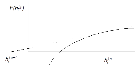
The solution to the second part of the right hand side of Equation 2.54 is referred to as the Newton-step \(\Delta h_i^{j+1,p}\):
\[ \left( \begin{array}{c} h_\text{1}^{j+1,p+1} \\ ⋮\\ h_{i}^{j+1,p+1} \\ ⋮\\ h_{n}^{j+1,p+1} \\ \end{array} \right) = \left( \begin{array}{c} h_\text{1}^{j+1,p} \\ ⋮\\ h_{i}^{j+1,p} \\ ⋮\\ h_{n}^{j+1,p} \\ \end{array} \right) + \lambda \left( \begin{array}{c} h_\text{1}^{j+1,p} \\ ⋮\\ h_{i}^{j+1,p} \\ ⋮\\ h_{n}^{j+1,p} \\ \end{array} \right) \tag{2.55}\]
We always first try the full Newton step and we check at each iteration that the proposed step reduces \(0.5\sum_{i=1}^{n} F_{i}^\text{2}\). If not, we backtrack along the Newton direction until we have an acceptable step. The aim is to find \(\lambda\) which results in a decrease of \(0.5\sum_{i=1}^{n} \left[F_{i}\left(h_{i}^{j+1,p} + \lambda \Delta h_{i}^{j+1,p}\right)\right]^2\). The first estimate of \(\lambda\) amounts to 1. If it is decided that a second estimate is needed, \(\lambda\) is set to 1/3. The third estimate amounts to 1/9. Thereafter, no further reduction of \(\lambda\) is applied but a new Newton-iteration step is performed.
In SWAP the main convergence criterium in the unsaturated zone is based on the water closure term of the water balance \(F\). If \(\left|F_{i}\right|\) is less than a user defined criterion for all compartments, it is decided that the iteration cycle has resulted into a sufficiently accurate solution.
Numerical implementation of the top and bottom boundary conditions is described in Appendix E.
2.5 User instructions
2.5.1 General
Tip 2.1 shows the general input of soil water flow. The initial soil moisture condition (Part 1) is defined by the soil water pressure head. Initial values can by specified as function of soil depth with linear interpolation between depths (swinco = 1; htb) or can be calculated assuming hydrostatic equilibrium with a groundwater level (swinco = 2; gwli). A third option is to use the output of an earlier SWAP simulation (swinco = 3; inifil). This option is very useful when no data are available of the initial soil moisture condition.
Part 4 describes the vertical discretization of the soil profile. In addition to the natural soil layers with different hydraulic functions, the thicknesses of the calculation compartments should be defined. For correct simulation of infiltration and evaporation fluxes near the soil surface, the compartment thickness near the soil surface should be \(\le\) 1 cm. Deeper in the soil profile, where the soil water flow is less dynamic, the compartment thicknesses may increase (to 10 or more cm). In Part 5 the hydraulic parameters of each distinct soil layer are defined, which describe the water retention and hydraulic conductivity functions. The use of the air-entry-value concept \(h_e\) requires special care. Even a small value of \(\left|h_e\right|\) can cause a large change in \(K\left(\theta \right)\) of fine-textured soils (see Section 2.2.2). In fact, the use of the air-entry-value concept requires the re-fitting of the other parameters of the classical Mualem-Van Genuchten model on the original experimental data. In case the soil hydraulic functions are provided as tables (swsophy = 1), for each soil layer a separate file should be provided. Each file should provide the following column-oriented data: headtab (for \(h\)), thetatab (for \(\theta\)) and [conductab]{var} (for \(K\)). Due to the interpolation method, the outcome does depend on the user-supplied information in the input tables. Best results are obtained when the \(h\)-\(\theta\)-\(K\) tables contain many data points nicely distributed over all variables (e.g., based on equal log-transformed \(h\) interval (e.g., 0.1), or a dense grid of effective degree of saturation), with special attention to data close to saturation and data close to wilting point and beyond (see example in Tip 2.2). For example, in case the user has data available measured in the laboratory it is advised to first describe these data by some kind of analytical expression, and then derive tables based on this analytical expression. Experience has shown that supplying a coarse (or irregular) grid of \(h\)-\(\theta\)-\(K\) data points may cause unrealistic behaviour of the interpolated results, e.g. in the derivation of \(C\).
The piecewise cubic Hermite interpolation requires information regarding the behaviour at the end-points of the tabulated data. Currently, this is internally defined as provided in Table 2.2. The current pre-defined behaviour at the end-points is in agreement with the analytical behaviour of the Mualem-van Genuchten relationships. In case other relationships are used, this behaviour might be in conflict with these pre-defined characteristics. In a future release this might be solved by giving the user the opportunity to supply endpoint behaviour as input.
| End point in h | Retention | Conductivity | Comment |
|---|---|---|---|
| h = 0 | dθ/dh = 0 | d2K/dh2 = 0 | Data for h = 0 must be provided |
| h → ∞ | d2 θ/dh2 = 0 | d2K/dh2 = 0 | Thus data for a very large negative value should be provided |
In Part 6 the inclusion of hysteresis in the water retention function can be chosen. This option can only be chosen in combination with the Mualem van Genuchten parameterisation of the soil hydraulic properties. In case of hysteresis, also the parameter alfaw of the wetting curve (Part 5) should be defined. Whether the initial condition is wetting or drying, can have some impact on the simulation results in the first part of the simulation period. The duration of this period increases with the depth to the groundwater level. We advise only to implement hysteresis to the shallow layers (till max. 1,5 m below the soil surface), because deep unsaturated layer will probably slowly tend to the main wetting curve resulting in unexpected effects on the water balance. The change from drying to wetting scanning curve and vice versa depends on the relative cumulative \(\Delta h\) since the last check (parameter tau). The parameter tau is usually set equal to 0.01 cm. This means that the need for change of scanning curve is performed 100 times per pF unit. Because hysteresis is implemented explicitly we advise to set the maximum timestep DTMAX to 0.001 d. To gain insight into which maximum timestep should be used, a number of calculations can be made with DTMAX = 10-5, 10-4, 10-3 to determine which maximum timestep still produces similar results as those at the smallest time step. The parameter maxbacktris set to 6 in case of hysteresis (usually 3).
In Part 9 various parameters are defined that may affect the numerical solution of the Richards equation. In general, the default values will garantee an accurate numerical solution of the Richards equation for common soil profiles. In extreme hydrologic or textural cases adjustment of the default values might be required. The user should specify a minimum and a maximum time step, \(\Delta t_{min}\) and \(\Delta t_{max}\) (d; respectively dtmin and dtmax). SWAP will determine the optimal time step which minimizes the computational effort of a simulation while the numerical solution still meets the convergence criteria. For this purpose, SWAP employs the number of iterations needed to reach convergence, \(N_{it}\), in the following way (Kool and Genuchten (1991)):
- \(N_\text{it}\) < 3 : multiply time step with a factor 2
- 3 \(\le\) \(N_\text{it}\) \(\le\) \(N_\text{max}\) : keep time step the same
- \(N_\text{it}\) > \(N_\text{max}\) : divide time step by a factor 2
where \(N_\text{max}\) is the defined maximum number of iterations (maxit; default 30). Also the maximum number of back-track cycles should be specified by the user (maxbacktr). A common value for this maximum is 5.
Routinely, SWAP uses 4 convergence criteria:
- the water balance error of each soil compartment: should be less than 10-6 cm
- between iterations the relative difference in pressure head (-) per compartment should be less than a user specified criterion (critdevh1cp, e.g. 10-2)
- between iterations the absolute difference in pressure head (cm) per compartment should be less than a user specified criterion (critdevh2cp, e.g. 10-1 cm)
- the water balance error of a possible ponding layer should be less than a user specified criterion (critdevpondt, e.g. 10-4 cm)
In addition, SWAP will give a warning when groundwater levels between time steps fluctuate more than a user specified criterion (gwlconv).
For the initial time step, SWAP will take \(\Delta t = \sqrt{\Delta t_\text{min} \Delta t_\text{max}}\). Depending on \(N_\text{it}\), the time step will be decreased, maintained or increased for the following time steps as described above. The time step is always confined to the range \(\Delta t_\text{min} \le \Delta t \le \Delta t_\text{max}\). When the actual time step during simulation reaches its minimum value (\(\Delta t = \Delta t_\text{min}\)), the maximum number of iterations is expanded to 2 * \(N_\text{max}\). If still the numerical solution shows no convergence, SWAP prints a warning in the *.wrn file, and continues the simulation at the next time step with the pressure heads of the last iteration.
In Part 9 also a choice can be made with respect to spatial averaging of hydraulic conductivity and updating hydraulic conductivity in the numerical solution. Default choices are weighted arithmetic mean (swkmean = 2) and no update of hydraulic conductivity (swkimpl = 0) (see also Section 2.4.1).
2.5.2 Bottom boundary conditions
SWAP offers various options to prescribe the lower boundary condition, each having their typical scale of application (see Table 2.3 and Tip 2.3).
| Lower boundary condition | Description | Type of condition | Typical scale of application |
|---|---|---|---|
| 1 | Prescribe groundwater level | Dirichlet | field |
| 2 | Prescribe bottom flux (qbot) | Neumann | region |
| 3 | Calculate bottom flux from hydraulic head of deep aquifer | Cauchy | region |
| 4 | Calculate bottom flux as function of groundwater level | Cauchy | region |
| 5 | Prescribe soil water pressure head of bottom compartment | Dirichlet | field |
| 6 | Bottom flux equals zero | Neumann | field / region |
| 7 | Free drainage of soil profile | Neumann | field |
| 8 | Free outflow at soil-air interface (seepage face) | Neumann / Dirichlet | field |
In case of options 1, 2, 3, 5 and 6, in addition to the flux across the bottom of the modelled soil profile (\(q_\text{bot}\)), a drainage flux (\(q_\text{drain}\)) can be defined (Chapter 4). In case of option 4, the lower boundary includes drainage to local ditches or drains so \(q_\text{drain}\) should not be defined separately. In case of options 7 and 8, the simulated soil profile is unsaturated, so lateral drainage will not occur. We will discuss the 8 available bottom boundary conditions sequentially.
1. Prescribed groundwater levels
In this case a field-averaged groundwater level (\(\phi_\text{avg}\)) is given as a function of time (Tip 2.3). SWAP will linearly interpolate between the dates and times at which the groundwater levels are specified. SWAP will read times according to the following format: 05-jan-2005_14:30:00.00 denotes January 5, 2005 at 2.30 PM. If only dates and no times are specified (as in Tip 2.3), SWAP will assume time 0:00.
The main advantage of this boundary condition is the easy recording of the phreatic surface in case of a present groundwater table. A drawback is that at shallow groundwater tables the simulated phreatic surface fluctuations are very sensitive to the soil hydraulic functions and the top boundary condition. If the top and bottom boundary condition not match accurately, or the soil hydraulic functions deviate from reality, strong fluctuations of simulated water fluxes across the lower boundary may result. Especially when the output of SWAP is used as input in water quality calculations, it is recommended to use another type of lower boundary condition. The option of prescribed groundwater levels is disabled for macropore flow simulations.
Experience has shown that SWAP cannot correctly handle this boundary condition in case the (interpolated) prescribed groundwater level is inside frozen soil. An alternative boundary condition to achieve approximately the desired groundwater levels is to impose pressure heads at the bottom of the simulated soil profile which are in hydrostatic equilibrium with the desired phreatic surface (option 5).
2. Prescribed bottom flux
In this case the bottom flux (\(q_\text{bot}\)) might be given as function of time with linear interpolation between the data pairs, or as a sine function (Tip 2.3). This option has a similar disadvantage as the previously described option with the prescribed groundwater level at the field scale. When a mismatch occurs between boundary conditions (e.g. drainage + leakage to deep aquifer exceeds net precipitation excess) the result may be a continuously declining or increasing groundwater level. In particular in cases where the output of SWAP is used as input in water quality calculations, it is recommended to use another type of lower boundary condition.
3. Calculate the bottom flux from the hydraulic head of a deep aquifer
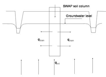
Figure 2.4 shows a soil profile which is drained by ditches and which receives a seepage flux from a semi-confined aquifer. SWAP makes a distinction between \(q_\text{drain}\), the local drainage flux to ditches and drains (see Chapter 4), and \(q_\text{bot}\), the bottom flux due to regional groundwater flow.
The bottom flux \(q_\text{bot}\) depends on the average groundwater level \(\phi_\text{avg}\) (cm), the hydraulic head in the semi-confined aquifer \(\phi_\text{aquif}\) (cm), and the resistance of the semi-confining layer \(c_\text{1}\) (d):
\[ q_\text{bot} = \frac{\phi_\text{aquif} - \phi_\text{avg}} {c_\text{1} + \sum_{i=i_\text{gwl}}^{n} \frac{\Delta z_\text{i}}{K_\text{sat,i}}} \tag{2.56}\]
where the subscript \(i_\text{gwl}\) points to the compartment number in which the groundwater level is located. The vertical resistance between the bottom of the model and the groundwater level may be taken into account by adding it to the aquitard resistance \(c_\text{1}\). The hydraulic head \(\phi_\text{aquif}\) is prescribed using a sinusoidal wave:
\[ \phi_\text{aquif} = \phi_\text{aquif,m} + \phi_\text{aquif,a} \cos \left(\frac{2\pi}{phi_\text{aquif,p}} \left(t-t_\text{max}\right) \right) \tag{2.57}\]
where \(\phi_\text{aquif,m}\) , \(\phi_\text{aquif,a}\) , and \(\phi_\text{aquif,p}\) are the mean (cm), amplitude (cm) and period (d) of the hydraulic head sinus wave in the semi-confined aquifer, and \(t_\text{max}\) is the time (d) at which \(\phi_\text{aquif}\) reaches its maximum.
SWAP includes the option for the implicit treatment of pressure head in lowest compartment by substitution of \(\phi_\text{avg}\) by \(h_\text{n}^\text{j+1}+z_\text{n}\) and considering the vertical resistance within the model domain only between the lowest node and the lower boundary. Another option involves the possibility to specify a groundwater flux additional to \(q_\text{bot}\) to facilitate the coupling of the SWAP model to a regional groundwater model.
4. Calculate bottom flux as a function of groundwater level
The relation between \(q_\text{bot}\) and \(\phi_\text{avg}\) can be given as an exponential relation or as a table (Tip 2.3). The exponential relationship is formulated as:
\[ q_\text{bot} = a_\text{qbot} \exp \left( b_\text{qbot} \left| \phi_\text{avg} \right| \right) + c_\text{qbot} \tag{2.58}\]
where \(a_\text{qbot}\) (cm d-1), \(b_\text{qbot}\) (cm-1) and \(c_\text{qbot}\) (cm d-1) are empirical coefficients. This type of exponential relationship was derived for deep sandy areas in the eastern part of The Netherlands (Massop and Wit 1994). Special care should be taken with respect to the distinction between drainage and bottom boundary flux. The relationship that may be used to compute drainage (Chapter 4) can conflict with the relation for \(q_\text{bot}\). It may then be appropriate to apply another type of boundary condition. When the relation between \(q_\text{bot}\) and \(\phi_\text{avg}\) is given as a table, \(q_\text{bot}\) results from an interpolation between groundwater level and bottom flux listed in the table, using the simulated groundwater level (\(\phi_\text{gwl}\)).
5. Prescribed soil water pressure heads at the bottom of the model
In this case values of \(h_\text{bot}\) should be specified as function of time. For times between observations, SWAP will interpolate linearly.
6. Zero flux at the bottom of the model domain
A bottom flux (\(q_\text{bot}\)) of zero may be applied when an impervious layer exists at the profile bottom or when groundwater flow below the profile bottom can be neglected. This option is implemented with a simple switch, which forces \(q_\text{bot}\) to zero.
7. Free drainage
In case of free drainage, the total hydraulic head \(H\) gradient is assumed to be equal to one at the bottom boundary, which sets \(q_\text{bot}\) equal to the hydraulic conductivity of the lowest compartment:
\[ \frac{\partial H}{\partial z}=1 \quad \text{thus:} \quad q_\text{bot} = -K_n \tag{2.59}\]
8. Free outflow (seepage face)
In this case, drainage will only occur if the pressure head in the bottom compartment (\(h_\text{n}\)) becomes larger than zero. During drainage and after a drainage event, hn is set equal to zero and \(q_\text{bot}\) is calculated by solving the Richards equation. This option is commonly applied for lysimeters, where outflow only occurs when the lowest part of the lysimeter becomes saturated. In the field this condition is appropriate when the soil profile is drained by a coarse gravel layer. Lysimeters with groundwater table controlling provisions can also be simulated imposing a zero bottom flux condition (swbotb = 6), combined with a single drainage system, where the drainage resistance is low.
2.5.3 Instructions for Peters - Durner - Iden
The use of either of the 8 PDI models cannot be considered together with hysteresis, macropore flow or a user-supplied air entry value.
In the example below the parameters for a scaled bimodal PDI model (ihwckmodel = 11) are provided for a soil consisting of two layers. There is no restriction of the type of model for each layer: they may be different.
By default, ihwckmodel = 1, indicating that the standard MvG model is used. So, if the variable ihwckmodel is not present then the standard MvG model is used. Note that ihwckmodel = 2 or 3 are special cases for technical testing only, and should not be used by the user.