| CO2 (ppm) | Amax | εPAR | Tp | Amax | εPAR | Tp |
|---|---|---|---|---|---|---|
| 40 | 0.0 | 0.00 | 0.0 | 0 | 0 | 0.00 |
| 360 | 1.0 | 1.00 | 1.0 | 1 | 1 | 1.00 |
| 720 | 1.6 | 1.11 | 0.9 | 1 | 1 | 0.74 |
| 1000 | 1.9 | 1.11 | 0.9 | 1 | 1 | 0.74 |
| 2000 | 1.9 | 1.11 | 0.9 | 1 | 1 | 0.74 |
7 Crop growth
7.1 Introduction
SWAP includes two crop growth modules: a simple module for static crop growth and a detailed module for dynamic crop growth, covering arable crops (WOFOST, WOrld FOod STudies) as well as grass (re)growth. Static crop growth assumes a fixed development of leaf area index and rooting depth, independent of climatic conditions, whereas dynamic crop growth responds to climatic conditions and is influenced by stress factors.
SWAP enables various types of land use to rotate over time. A sequence with combinations of different crop modules is hereby allowed. For each crop the user should specify the cropping period (see Section 7.2).
The main function of the simple module for static crop growth is to provide proper upper boundary conditions for soil water movement. The simple model is useful when crop growth doesn’t need to be simulated or when crop growth input data are insufficient. Section 7.3 provides a description of the simple module.
In the footsteps of De Wit and co-workers (De Wit 1978; Goudriaan 1977; Penning de Vries and Laar 1982), in the 1980s a wide range of scientists in Wageningen became involved in the development and application of dynamic crop growth models. The generic crop model SUCROS for the potential production situation was developed Spitters, Keulen, and Kraalingen (1989). SUCROS formed the basis of a range of Wageningen crop models, as reviewed by Bouman et al. (1996) and Van Ittersum et al. (2003). One of the developed models is the WOFOST model, which simulates in detail photosynthesis and crop development, taking into account growth reductions due to water and/or salt stress. WOFOST has been implemented in SWAP and is described in Section 7.4.
Several approaches for simulating root growth are available (see Section 7.5), and Section 7.6 describes the option for modelling the effect of changes in atmospheric CO2 on crop development.
7.2 Cropping period
The cropping period indicates the maximum duration of crop growth activity. The actual period is depending on the crop emergence and, for arable crops, the timing of harvest. Dynamic crop growth models use initial values for the total crop dry weight and the leaf area index at emergence. If emergence of an arable crop is delayed, bare soil conditions are maintained. For grassland the initial values are maintained until growth starts.
7.2.1 Arable Crops
The moment of emergence can be delayed due to unfavourable hydrological conditions affecting field workability or due to germination constraints. The end of the cropping period is determined by the timing of harvest.
Preparation
The first process which can delay the emergence of an arable crop is field preparation. Entering a field with heavy machinery, for instance in case of ploughing, is not always possible due to unfavourable hydrological conditions. If the pressure head at a specific depth is insufficient, field preparation is delayed. When the pressure head criterion is met, the sowing process can start.
Sowing
During the sowing process, the pressure head at a specific depth is monitored in a manner similar to field preparation. In addition, soil temperature is also monitored at a specified depth. Sowing takes place only when both the pressure head and soil temperature criteria are satisfied.
Germination
For germination, the method of Van Wijk et al. (1988) was implemented similar to Van Walsum and Bolt (2013). Germination depends on temperature:
\[ T_{\text{sum,germ}} = \begin{cases} T_{\text{sum,germ}} & \text{for} \space T_{\text{av}} < T_{\text{min,germ}}\\ T_{\text{sum,germ}} + \frac{T_{\text{sum,eme,opt}}}{T_{\text{sum,eme,sub}}} \left(T_{\text{av}} - T_{\text{min,germ}}\right) & \text{for} \space T_{\text{min,germ}} < T_{\text{av}} < T_{\text{max,germ}}\\ T_{\text{sum,germ}} + \frac{T_{\text{sum,eme,opt}}}{T_{\text{sum,eme,sub}}} \left(T_{\text{max,germ}} - T_{\text{min,germ}}\right) & \text{for} \space T_{\text{av}} > T_{\text{max,germ}} \end{cases} \tag{7.1}\]
where \(T_{\text{av}}\) is the mean daily air temperature (°C; average of the minimum and maximum temperature), \(T_{\text{min,germ}}\) is the minimum temperature for Tsum calculation (°C d), \(T_{\text{max,germ}}\) is the maximum temperature for Tsum calculation (°C d), \(T_{\text{sum,germ}}\) is the Tsum during the germination period (°C d), \(T_{\text{sum,eme,opt}}\) is the Tsum for crop emergence under optimal soil moisture and temperature conditions (°C d), and \(T_{\text{sum,eme,sub}}\) is the Tsum for crop emergence under sub-optimal soil moisture and temperature conditions (°C d).
Tsum for crop emergence under sub-optimal soil moisture and temperature conditions is calculated by:
\[ T_{\text{sum,eme,sub}} = \begin{cases} -a \log_{10}(-h_{\text{rz}}) + b & \text{for too wet conditions}\\ T_{\text{sum,eme,opt}} & \text{for optimal conditions}\\ a \log_{10}(-h_{\text{rz}}) + c & \text{for too dry conditions}\\ \end{cases} \tag{7.2}\]
where \(a\), \(b\), and \(c\) are parameters (with \(b\) and \(c\) determined by SWAP), and \(h_{\text{rz}}\) is the average pressure head of the upper 10 cm of the soil. Emergence occurs when:
\[ T_{\text{sum,germ}} > T_{\text{sum,eme,opt}} \tag{7.3}\]
Harvest
The timing of harvest defines the end of the cropping period. Optionally, harvesting can take place before the end of the cropping period if the crop is mature. After harvesting, bare soil conditions are assumed.
7.2.2 Grassland
The initialisation of grass growth has 2 options with different thresholds to start growth:
- Sum of air temperatures: Growth starts when the accumulated sum of positive daily air temperatures exceeds 200 °C.
- Soil temperature at a specific depth: Growth begins when the soil temperature at a given depth exceeds a defined threshold for a specified number of consecutive days.
7.3 Simple module for static crop growth
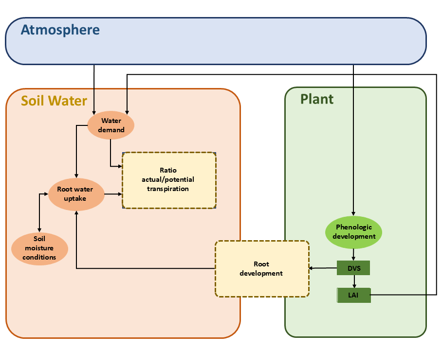
The simple crop growth model represents a green canopy that intercepts precipitation, transpires water vapor, and shades the ground. The user specifies crop variables as a function of the development stage. The variables to be specified are crop height, rooting depth, and either leaf area index or soil cover fraction. The development stage is controlled either by the temperature sum or can be linear in time. Atmospheric conditions together with the crop status drive water demand, which interacts with soil moisture and root water uptake to determine the ratio of actual to potential transpiration, see Figure 7.1.
Unlike dynamic crop growth models, static crop growth does not simulate the crop potential or actual yield. However, users can approximate yield by relating potential transpiration and transpiration reduction caused by stress factors, using the potential yield and yield response factors (Doorenbos and Kassam 1979; Smith 1992). The actual yield \(Y_{a}\) (kg ha-1) relative to the potential yield \(Y_{p}\) (kg ha-1) is calculated by:
\[ 1 - \frac{Y_{a}}{Y_{p}} = K_{y} \left(1 - \frac{T_{a}}{T_{p}}\right) \tag{7.4}\]
where \(K_{y}\) (-) is the yield response factor, and \(T_{p}\) (cm) and \(T_{a}\) (cm) are the potential and actual transpiration.
7.4 Detailed module for dynamic crop growth
Three groups of growth factors (Figure 7.2) can be distinguished to obtain a hierarchy of production levels in crop production (Van Ittersum et al. 2003). Growth-defining factors, such as radiation intensity, carbon dioxide concentration, temperature, and crop characteristics, determine the potential production that can be achieved in a given physical environment and for a given plant species. To achieve the potential production, the crop must be optimally supplied with water and nutrients and completely protected against weeds, pests, diseases, and other factors that may reduce growth.
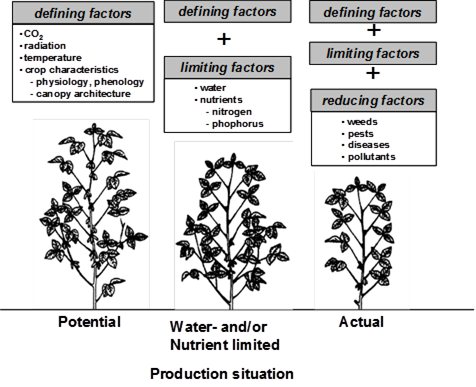
Growth-limiting factors such as water and nutrients determine the water- or nutrient-limited production level in a given physical environment. Through management of the water and nutrients availability, crop production may increase towards potential levels. Growth-reducing factors that reduce or hamper growth comprise biotic factors such as weeds, pests, and diseases, and abiotic factors such as pollutants. Crop protection aims at effective management of these factors. In the actual production situation, crop productivity is usually the result of a combination of growth-limiting and growth-reducing factors (Van Ittersum et al. 2003).
WOFOST (Van Keulen and Wolf 1986; Spitters, Keulen, and Kraalingen 1989; Supit, Hooyer, and Diepen 1994; Hijmans, Guiking-Lens, and Diepen 1994; Boogaard et al. 1998) simulates potential and limited production due to water and/or salinity and/or nutrient stress. Figure 7.3 shows the processes and relations incorporated in WOFOST. The energy that is absorbed by the canopy depends on the incoming radiation, the crop leaf area, and the photosynthetic leaf characteristics. With the absorbed radiation, the potential gross photosynthesis is calculated, which is subsequently reduced due to water/salinity/nutrient stress yielding the actual gross photosynthesis.
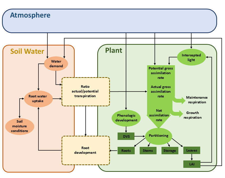
Part of the produced carbohydrates (CH2O) are used for the maintenance of the living biomass (maintenance respiration). The remaining carbohydrates are converted into structural matter. This conversion process costs energy and some weight is lost (growth respiration). The remaining dry matter is partitioned among roots, leaves, stems, and storage organs, using partitioning factors that are a function of the phenological development stage (Spitters, Keulen, and Kraalingen 1989). The fraction partitioned to the leaves determines leaf area development and hence the dynamics of light interception. Integrating the growth rates over time yields the dry weight of the crop organs. During the seasons, part of the living biomass dies due to senescence.
Light interception and CO2 assimilation are the main growth-driving processes. Some of these crop growth processes are influenced by temperature, like the maximum photosynthesis and the maintenance respiration rate. Other processes, like the assimilate partitioning and tissue decay, are a function of the phenological development stage (which is a function of the thermal time).
7.4.1 Phenological development stage
As many physiological and morphological processes change with the phenological stage, quantification of the phenological development is essential in any crop growth simulation model. For many annual crops, the phenological development can be expressed as a development stage \(D_s\) (-), having the value 0 at seedling emergence, 1 at flowering, and 2 at maturity (Van Heemst 1986a, 1986b). The most important phenological change is the one from the vegetative (\(0 < D_s < 1\)) to reproductive stage (\(1 < D_s < 2\)), which drastically changes the dry matter allocation to organs.
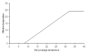
Crop growth simulation starts either at sowing or emergence. The sowing or emergence date should be specified by the user. A crop passes through successive phenological development stages, the length of which depends on the development rate. Development rates before floral initiation or anthesis (\(D_s = 1\)) are controlled by temperature and sometimes depend on day length as well. After anthesis, the development rate only depends on the temperature. Higher temperatures accelerate the development rate, leading to shorter growing periods. It has often been demonstrated that the development rate increases more or less linearly with temperature (Van Dobben 1962; Van Keulen and Seligman 1987). Therefore, WOFOST uses the temperature sum to describe the development stage. The temperature sum is calculated using the effective temperature \(T_{\text{eff}}\) (°C), which is a tabular function of the daily average temperature \(T_{\text{day}}\) (°C) (Figure 7.4). Generally, for species originating from temperate regions \(T_{\text{day}} - T_{\text{eff}} = 0-3\) °C, while for species of subtropical and tropical origins \(T_{\text{day}} - T_{\text{eff}} = 9-14\) °C (Angus et al. 1981). Note that \(T_{\text{eff}}\) cannot be negative. The user should specify \(T_{\text{eff}}(T_{\text{day}})\) and the relation between crop development stage \(D_s\) and \(T_{\text{eff}}\):
\[ D_s^{(j+1)} = D_s^j + \frac{T_{\text{eff}}}{T_{\text{sum,i}}} \tag{7.5}\]
where superscript \(j\) is the day number and \(T_{\text{sum,i}}\) is the temperature sum required to complete either the vegetative or the reproductive stage. Within a species, cultivars may vary substantially in their temperature requirements.
For some species or cultivars, the day length during the vegetative stage should be accounted for. Approaches that describe such effects quantitatively are given, among others, by Weir et al. (1984), Hadley et al. (1984), and Reinink, Jorritsma, and Darwinkel (1986). In WOFOST, a reduction factor for the development rate as a function of day length \(f_{\text{lday}}\) (-) is computed:
\[ f_{\text{lday}} = \frac{L_{\text{day}} - L_{\text{cday}}}{L_{\text{oday}} - L_{\text{cday}}} \quad \text{with} \quad 0 < f_{\text{lday}} < 1 \tag{7.6}\]
with \(L_{\text{day}}\) the actual day length (d), \(L_{\text{cday}}\) the critical day length for development (d), and \(L_{\text{oday}}\) the optimum day length for development (d). The critical and the optimum day length should be provided by the user. Note that in modern cultivars, photosensitivity is much less pronounced than in traditional cultivars, and the day length influence can be ignored by choosing an appropriate temperature sum, which leads to an equivalent crop life cycle.
Crop growth simulation stops when the development stage reaches ripeness (\(D_s = 2\)) or when the crop will be harvested (i.e., before ripeness). In this later case, the user should specify the harvest date.
7.4.2 Radiation fluxes above the canopy
Measured or estimated daily global radiation (wavelength range 300 - 3000 nm) is input for the model. Incoming radiation is partly direct, with the angle of incidence equal to the angle of the sun, and partly diffuse, with incidence under various angles. The sine of solar elevation as a function of the day hour can be calculated with:
\[ \sin \beta_{\text{sun}} = \sin L_g \sin \sigma_{\text{sun}} + \cos L_g \cos \sigma_{\text{sun}} \cos \left( \frac{2\pi(t_h+12)}{24} \right) \tag{7.7}\]
with \(\beta_{\text{sun}}\) as the solar elevation (degrees), \(\sigma_{\text{sun}}\) as solar declination (degrees), \(L_g\) as geographic latitude (degrees), and \(t_h\) as hour of the day. Integration of \(\sin \beta_{\text{sun}}\) over the day and multiplication with the solar constant yields the daily extra-terrestrial radiation, which is also known as the Angot radiation (J m-2 d-1):
\[ R_o = S_c \int \sin \beta_{\text{sun}} \, dt \tag{7.8}\]
The solar constant \(S_c\) (J m-2 d-1) can be calculated as:
\[ S_c = 1370 \left(1 + 0.033 \cos \left( \frac{2j\pi}{365} \right) \right) \tag{7.9}\]
where \(j\) is the day number in the year (DOY). Only about 50 percent of the global radiation is photosynthetically active (\(PAR\), Photosynthetically Active Radiation, wavelength band 400-700 nm). The daily incoming \(PAR\) (J m-2 d-1) is calculated by multiplying half of the daily global radiation with the ratio of the actual effective solar elevation and the integral of the effective solar height, taking into account reduced atmospheric transmission at low solar elevations:
\[ PAR = 0.5 R_g \frac{\sin \beta_{\text{sun}} (1 + 0.4 \sin \beta_{\text{sun}})}{\int \sin \beta_{\text{mod,sun}}} \tag{7.10}\]
where \(R_g\) is daily global radiation (J m-2 d-1) and \(\int \sin \beta_{\text{mod,sun}}\) is the integral of \(\sin \beta_{\text{sun}}\) over the day (-) which is corrected for reduced atmospheric transmission at low solar elevations (Spitters, Toussaint, and Goudriaan 1986).
The diffuse radiation flux results from scattering of sun rays by clouds, gases, and dust in the atmosphere. To quantify the diffuse radiation, first the atmospheric transmission is calculated as:
\[ T_{\text{atm}} = \frac{R_g}{R_o} \tag{7.11}\]
The relation between the proportion of the diffuse flux in the global irradiance (\(R_{\text{df}}/R_g\)) and the atmospheric transmission \(T_{\text{atm}}\) is characterized by an approximately linear trend for transmissions ranging between 0.35 and 0.75. At low transmissions, nearly all of the incoming radiation is diffuse so that the curve bends off. There is some variation among published relations, arising from differences in atmospheric conditions, especially relative sunshine duration, water content of the atmosphere, and cloud type, but also lack of fit of the presented regression equation from the data and differences in the method of measuring the diffuse radiation. The relation used in WOFOST has been derived by De Jong (1980) and has been recommended by Spitters, Toussaint, and Goudriaan (1986):
\[ \frac{R_{\text{df}}}{R_g} = \begin{cases} 1 & \text{for} \space T_{\text{atm}} \leq 0.07 \\ 1 - 2.3 (T_{\text{atm}} - 0.07)^2 & \text{for} \space 0.07 < T_{\text{atm}} \leq 0.35 \\ 1.33 - 1.46 T_{\text{atm}} & \text{for} \space 0.35 < T_{\text{atm}} \leq 0.75 \\ 0.23 & \text{for} \space T_{\text{atm}} > 0.75 \end{cases} \tag{7.12}\]
The diffuse photosynthetically active radiation \(PAR_{\text{dif}}\) (J m-2 d-1) can be calculated by:
\[ PAR_{\text{dif}} = 0.5 \frac{R_{\text{df}}}{R_g} T_{\text{atm}} R_o \tag{7.13}\]
The direct radiation flux, \(PAR_{\text{dir}}\) (J m-2 d-1), is obtained by subtracting the diffuse part from the photosynthetically active radiation flux:
\[ PAR_{\text{dir}} = PAR - PAR_{\text{dif}} \tag{7.14}\]
7.4.3 Radiation profiles within the canopy
The incoming \(PAR\) is partly reflected by the canopy. The reflection coefficient is defined as the fraction of the downward radiation flux that is reflected by the entire canopy. The reflection coefficient \(\rho_{\text{rad}}\) (-) of a green leaf canopy with a random spherical leaf angle distribution equals (Goudriaan 1977):
\[ \rho_{\text{rad}} = \left( \frac{1 - \sqrt{1 - \sigma_{\text{leaf}}}}{1 + \sqrt{1 - \sigma_{\text{leaf}}}} \right) \left( \frac{2}{1 + 1.6 \sin \beta_{\text{sun}}} \right) \tag{7.15}\]
with \(\sigma_{\text{leaf}}\) the scattering coefficient of single leaves for visible radiation (-), which is set to 0.2 (Goudriaan 1977). The first right-hand-side term of Equation 7.15 denotes the reflection of horizontal leaves and the second term is the approximate correction factor for a spherical leaf angle distribution. The fraction \((1 - \rho_{\text{rad}})\) of the incoming visible radiation is available for absorption by the canopy.
Light intensity, adjusted for crop reflection, decreases approximately exponentially with leaf area index when going deeper into the canopy:
\[ PAR_L = (1 - \rho_{\text{rad}}) PAR e^{-\kappa L} \tag{7.16}\]
where \(L\) is the cumulative leaf area index, \(\Sigma LAI\) (m2 leaf m-2 ground), counted from the top of the canopy downwards, \(PAR_L\) is the net light intensity (J m-2 d-1) at depth \(L\), and \(\kappa\) is the radiation extinction coefficient (-).
The profiles of the net diffuse flux and the net flux caused by direct irradiance can be characterized analogously (Goudriaan 1982). Diffuse and direct fluxes each attenuate at a different rate, and both extinction coefficients are input in SWAP. For a random spherical leaf angle distribution, the extinction coefficient of the direct flux component, \(\kappa_{\text{dir}}\) (-), might be approximated by (Goudriaan 1977, 1982):
\[ \kappa_{\text{dir}} = \frac{0.5}{\sin \beta_{\text{sun}}} \tag{7.17}\]
and the extinction coefficient of the diffuse flux component, \(\kappa_{\text{dif}}\) (-), might be calculated as:
\[ \kappa_{\text{dif}} = \kappa_{\text{dir}} \sqrt{1 - \sigma_{\text{leaf}}} \tag{7.18}\]
In Equation 7.17, the factor 0.5 represents the average projection on the ground surface of leaves showing a spherical angle distribution. Averaging \(0.5/\sin \beta\) during a day with an overcast sky, gives a value of \(\kappa_{\text{dir}} = 0.8\) (-). The value of \(\kappa_{\text{dif}}\) can be measured directly under completely overcast sky conditions, when only diffuse radiation reaches the canopy. The average value is about 0.72 (-) (Goudriaan 1977).
In many situations, the leaf angle distribution is not spherical. Therefore, in WOFOST the actual leaf angle distribution is accounted for by using a so-called cluster factor, which is the measured extinction coefficient for diffuse radiation, relative to the theoretical one for a spherical leaf area distribution.
On its way through the canopy, part of the direct flux is intercepted and scattered by the leaves. Hence, the direct flux segregates into a diffuse, scattered component and another component which remains direct. Attenuation of the remaining direct component proceeds like in a hypothetical canopy of black, non-scattering leaves. The diffuse component is obtained as the difference between the total direct flux and its direct component. The light absorption rate at depth \(L\) in the canopy, \(PAR_{L,a}\) (J m-2 leaf d-1), is the derivative of Equation 7.16 with respect to \(L\):
\[ PAR_{L,a} = \kappa (1 - \rho_{\text{rad}}) PAR e^{-\kappa L} \tag{7.19}\]
Similar expressions can be derived for the separate light components: the diffuse flux, the total direct radiation flux, and the direct component of the direct radiation flux. The absorbed diffuse component of the direct flux is obtained by subtracting the direct component from the total direct flux.
7.4.4 Instantaneous assimilation rates per leaf layer
The canopy CO2 assimilation rate layer is obtained by substituting the absorbed amount of light energy into the assimilation-light response of single leaves (Peat 1970):
\[ A_L = A_{\text{max}} \left( 1 - e^{\frac{-\epsilon_{\text{PAR}} \cdot PAR_{(L,a)}}{A_{\text{max}}}} \right) \tag{7.20}\]
where \(A_L\) is the gross assimilation rate at relative depth \(L\) (kg CO2 m-2 leaf d-1), \(A_{\text{max}}\) the gross assimilation rate at light saturation (kg CO2 m-2 leaf d-1), and \(\epsilon_{\text{PAR}}\) the initial slope or light use efficiency (kg CO2 J-1 absorbed).
Two leaf classes are distinguished: shaded leaves and sunlit leaves. The shaded leaf area absorbs the diffuse flux and the diffuse component of the direct flux. The sunlit leaf area receives diffuse and direct radiation. At every horizon within the canopy, the intensity of the unobstructed direct beam equals its intensity above the crop. Illumination intensity of sunlit leaves varies strongly with leaf angle. In the model, the assimilation rate of the sunlit leaf area is therefore integrated over the leaf angle distribution.
The assimilation rate per unit leaf area in a canopy is the sum of the assimilation rates of sunlit and shaded leaves, taking into account their proportion in each layer. The proportion of sunlit leaf area at depth \(L\) in the canopy equals the proportion of the direct component of the direct flux reaching that depth. This proportion is calculated analogous to Equation 7.15, using the extinction coefficient of the direct radiation component.
Figure 7.5 shows the CO2 assimilation rate at different sunlight intensities as measured for various crops. Striking are the higher assimilation rates of so-called C4 crops in comparison to C3 crops. The reason is that C4 plants are more effective in CO2 fixation within a leaf (Moene and Dam 2014).
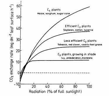
At a certain light intensity, the CO2 uptake rate and the photosynthesis are much higher in case of C4 plants.
7.4.5 Daily gross assimilation rate of the canopy
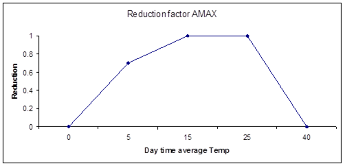
The maximum instantaneous CO2 assimilation rate \(A_{\text{max}}\) (kg CO2 ha-1 d-1) is crop and development stage dependent and should be provided by the user as a function of development stage. \(A_{\text{max}}\) has to be corrected for the atmospheric CO2 concentration and for the average daytime temperature \(T_{\text{day}}\) (°C) according to:
\[ A_{\text{pgross}}^1 = f_{\text{CO2}} f_{\text{tday}} A_{\text{max}} \tag{7.21}\]
where \(f_{\text{CO2}}\) is the [CO2] dependent correction factor and \(f_{\text{tday}}\) is the average daytime temperature that corrects \(A_{\text{max}}\) for sub-optimum temperatures. Both correction factors are crop specific and should be provided by the user as tables. The average daytime temperature \(T_{\text{day}}\) (°C) is calculated as:
\[ T_{\text{day}} = 0.75 \, T_{\text{max}} + 0.25 \, T_{\text{min}} \tag{7.22}\]
Figure 7.6 shows a typical occurrence of the daytime dependent correction factor.
In a next step, the instantaneous rates per leaf layer are integrated over the canopy leaf area index and over the day using the Gaussian integration method (Press et al., 1989). This method specifies the discrete points at which function values have to be calculated, and the weighting factors with which the function values have to be multiplied in order to minimize deviation from analytical integration. A three-point algorithm evaluates the function at 0.1127\(a\), 0.5\(a\) and 0.8873\(a\) of the interval (0,\(a\)), with weighting coefficients 1.0, 1.6 and 1.0, respectively. The Gaussian integration method is remarkably accurate in the case of trigonometric (radiation) and exponential (light absorption) functions. WOFOST computes at three selected moments of the day incoming \(PAR\) just above the canopy. Using this radiation, assimilation is computed at three selected depths in the canopy (Spitters, Keulen, and Kraalingen 1989). Gaussian integration of these values results in the daily gross CO2 assimilation rate, \(A_{\text{pgross}}\) (kg CO2 ha-1 d-1).
For each kg of absorbed CO2, 30/44 kg biomass (CH2O) is formed. Factors that reduce the daily assimilation rate are unfavorable temperatures, water shortage or excess and salinity stress:
\[ A_{\text{gross}} = \frac{30}{44} f_{\text{7min}} \left( \frac{T_a}{T_p} \right) A_{\text{pgross}}^1 \tag{7.23}\]
where \(A_{\text{gross}}\) is the daily gross assimilation rate (kg ha-1 d-1), \(f_{\text{7min}}\) is stress caused by low temperatures. At night, assimilates produced during the daytime are transformed into structural biomass. This process is hampered by low temperatures. If these low temperatures prevail for several days, the assimilation rate diminishes and ultimately halts. In WOFOST, \(f_{\text{7min}}\) is a function of the minimum temperature during the previous seven days. \(T_p\) is the potential transpiration, and \(T_a\) is the actual transpiration reduced by water, oxygen, salinity, and frost stress (see Section 3.5).
7.4.6 Maintenance respiration
Some of the carbohydrates formed are respired to provide energy for maintaining the existing bio structures. This maintenance respiration consumes roughly 15 - 30% of the carbohydrates produced by a crop in a growing season (Penning de Vries, Witlage, and Kremer 1979). This underlines the importance of accurate quantification of this process in the model.
WOFOST estimates the maintenance costs using the approach proposed by Penning de Vries and Laar (1982), assuming that the reference maintenance requirements \(R_{\text{mref}}\) (kg ha-1 d-1) are proportional to the dry weights of the plant organs to be maintained:
\[ R_{\text{mref}} = c_{\text{m,leaf}} W_{\text{leaf}} + c_{\text{m,stem}} W_{\text{stem}} + c_{\text{m,stor}} W_{\text{stor}} + c_{\text{m,root}} W_{\text{root}} \tag{7.24}\]
where \(c_{\text{m,i}}\) denotes the maintenance coefficient of organ \(i\) (kg kg-1 d-1) and \(W_i\) the organ dry weight (kg ha-1). The maintenance coefficients should be specified by the user.
The maintenance respiration rate still has to be corrected for senescence and temperature. The reduction factor for senescence \(f_{\text{senes}}\) (-) is crop-specific and is defined as a function of development stage. Higher temperatures accelerate the turnover rates in plant tissue and hence the costs of maintenance. An increase in temperature of 10°C increases maintenance respiration by a factor of about 2 (Kase and Catský 1984; Penning de Vries and Laar 1982). However, to be more flexible, the user may specify the increase factor of the respiration rate per 10°C temperature increase, \(Q_{10}\) (-):
\[ R_{\text{m}} = f_{\text{senes}} R_{\text{mref}} Q_{10}^{\frac{T_{\text{avg}} - 25}{10}} \tag{7.25}\]
where \(R_{\text{m}}\) is the actual maintenance respiration rate (kg ha-1 d-1).
It may be assumed that the vegetation will not be ‘self-consuming’ in terms of carbohydrates. Therefore, the maintenance respiration rate cannot exceed the gross assimilation rate. The net assimilation rate \(A_{\text{net}}\) (kg ha-1 d-1) is the amount of carbohydrates available for conversion into structural material:
\[ A_{\text{net}} = A_{\text{gross}} - R_{\text{m}} \quad \text{with} \quad A_{\text{net}} \geq 0 \tag{7.26}\]
7.4.7 Dry Matter Partitioning and Growth Respiration
The primary assimilates in excess of the maintenance costs are available for conversion into structural plant material. In this conversion process, CO2 and H2O are released. The magnitude of growth respiration is determined by the composition of the end product formed (Penning de Vries, Brunsting, and Laar 1974). Thus, the weight efficiency of conversion of primary photosynthates into structural plant material varies with the composition of that material. Fats and lignin are produced at high costs; structural carbohydrates and organic acids are relatively cheap. Proteins and nucleic acids form an intermediate group.
At higher temperatures, the conversion processes are accelerated, but the pathways are identical (Spitters, Keulen, and Kraalingen 1989). Hence, the assimilate requirements do not vary with temperature.
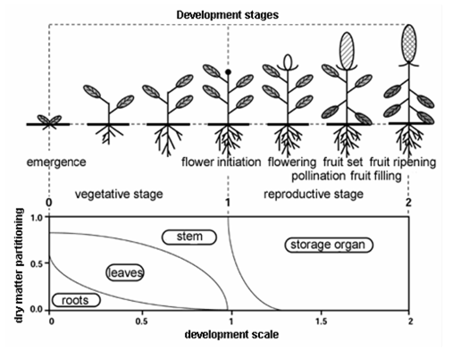
In the vegetative stage, the increase in total dry weight of the crop is partitioned over the plant organs: roots, leaves, stems, and storage organs. Storage organs, however, may not only be formed from current photosyntheses but also from carbohydrates and proteins that have been stored temporarily in vegetative parts and that are redistributed during the reproductive stage. In WOFOST, this redistribution process is not incorporated.
The partitioning factor depends on the crop development stage. Figure 7.7 gives a typical example. The partitioning factors are input to the model. WOFOST first divides the gross dry matter among roots and shoots (leaves, stems, and storage organs together), using the partitioning factor for roots, \(\xi_{\text{root}}\) (-). Next, WOFOST divides the gross dry matter directed to the shoots among leaves, stems, and storage organs, using the partitioning factors for these plant organs. At any development stage, the sum \(\xi_{\text{leaf}} + \xi_{\text{stem}} + \xi_{\text{stor}}\) must equal one.
For losses during conversion of general carbohydrates to specific plant tissues, average (crop-specific) conversion factors \(C_{\text{e,i}}\) (kg kg-1) should be specified for leaf, storage organ, stem, and root biomass. WOFOST calculates a weighted average, \(C_{\text{e}}\) (kg kg-1), of these organ-specific conversion factors by multiplying the organ-specific values with the partitioning factors:
\[ C_{\text{e}} = \frac{1}{\left(\frac{\xi_{\text{leaf}}}{C_{\text{e,leaf}}} + \frac{\xi_{\text{stor}}}{C_{\text{e,stor}}} + \frac{\xi_{\text{stem}}}{C_{\text{e,stem}}}\right) (1 - \xi_{\text{root}}) + \frac{\xi_{\text{root}}}{C_{\text{e,root}}}} \tag{7.27}\]
where \(\xi_i\) is the partitioning factor for organ \(i\).
The gross dry matter growth rate \(w_{\text{gross}}\) (kg ha-1 d-1) is related to the net assimilation rate \(A_{\text{net}}\) by:
\[ w_{\text{gross}} = C_{\text{e}} A_{\text{net}} \tag{7.28}\]
Gross dry matter growth is first partitioned between shoots (leaves, stems, and storage organs together) and roots:
\[ w_{\text{gross,root}} = \xi_{\text{root}} w_{\text{gross}} \quad \text{and} \quad w_{\text{gross,sh}} = (1 - \xi_{\text{root}}) w_{\text{gross}} \tag{7.29}\]
where \(\xi_{\text{root}}\) is the partitioning factor for roots (-) and \(w_{\text{gross,root}}\) and \(w_{\text{gross,sh}}\) are the gross growing rates (kg ha-1 d-1) of the roots and the shoots, respectively. The gross growth rate of leaves, stems, and storage organs is simply the product of the gross dry matter growth rate of the shoots and the fraction allocated to these organs.
7.4.8 Senescence
The death rate of storage organs is assumed to be zero. The death rate of stem and roots is crop specific and is defined as the daily amount of the living biomass that no longer participates in the plant processes. The death rate of stems and roots is considered to be a function of development stage as specified by the user.
The death rate of leaves is more complicated. Leaf senescence occurs due to water stress, shading (high LAI), and also due to exceedance of the life span.
The potential death rate of leaves due to water stress \(\zeta_{\text{leaf,water}}\) (kg ha-1 d-1) is calculated as:
\[ \zeta_{\text{leaf,water}} = W_{\text{leaf}} \left(1 - \frac{T_a}{T_p} \right) \zeta_{\text{leaf,p}} \tag{7.30}\]
where \(W_{\text{leaf}}\) is the leaf dry matter weight (kg ha-1), \(T_a\) and \(T_p\) are the actual and potential transpiration rates (cm d-1), respectively, and \(\zeta_{\text{leaf,p}}\) is the maximum relative death rate of leaves due to water stress (kg kg-1 d-1). The latter is crop specific and should be provided by the user.
A potential death rate due to self-shading, \(\zeta_{\text{leaf,shade}}\) (kg ha-1 d-1), is defined which increases linearly from zero at a critical leaf area index \(LAI_c\) (-) to its maximum value at \(2LAI_c\):
\[ \zeta_{\text{leaf,shade}} = 0.03 W_{\text{leaf}} \left( \frac{LAI - LAI_c}{LAI_c} \right) \quad \text{with} \quad 0 < \left( \frac{LAI - LAI_c}{LAI_c} \right) < 1 \tag{7.31}\]
with \(LAI_c = \frac{3.2}{\kappa_{\text{df}}}\). Typical values for \(\zeta_{\text{leaf,p}}\) and \(LAI_c\) are 0.03 d-1 and 4 m2m-2, respectively (Spitters, Keulen, and Kraalingen 1989).
WOFOST uses the highest value of \(\zeta_{\text{leaf,water}}\) and \(\zeta_{\text{leaf,shade}}\) for the combined effect of water stress and mutual shading.
Leaves that have escaped from premature death due to water stress or mutual shading inevitably die due to exceedance of the life span for leaves. Life span is defined as the maximum time a leaf can live at a constant temperature of 35°C. A physiologic aging factor, \(f_{\text{age}}\) (-), is calculated each day:
\[ f_{\text{age}} = \frac{T - T_{\text{b,age}}}{35 - T_{\text{b,age}}} \quad \text{with} \quad f_{\text{age}} \geq 0 \tag{7.32}\]
with \(T_{\text{b,age}}\) the lower threshold temperature for physiologic aging (°C), which is crop specific and should be provided by the user.
The integral of the physiologic aging factor over time yields the physiologic age, \(P_{\text{age}}\) (d):
\[ P_{\text{age}}^{(j+1)} = P_{\text{age}}^j + f_{\text{age}} \Delta t \tag{7.33}\]
To correct for leaf senescence, the specific leaf area of each day, \(SLA_j\) (ha kg-1), the growth of the dry matter weight of leaves per day, \(W_{\text{leaf}}\), and the physiological age, \(P_{\text{age}}\), are stored in 3 corresponding arrays. The first element of the arrays represents the most recent day, and the last element of the arrays represents the oldest day.
The leaf weight that died during a day due to water stress or mutual shading is subtracted from the weight of the oldest leaf class. When senescence is larger than the amount available in the oldest leaf class, the remaining senescence is subtracted from the next oldest leaf class. Emptying of the leaf classes continues until the amount of senescence is dissipated completely or the remaining amount of leaves becomes zero.
Leaves may maximally attain the age defined by the crop-specific life span. WOFOST checks the leaf class ages. The first class younger than the defined life span becomes the oldest class.
The stem death rate due to water stress is calculated in a similar way as the leaf death rate due to water stress using the same factor for the maximum relative death rate:
\[ \zeta_{\text{stem,water}} = W_{\text{stem}} \left(1 - \frac{T_a}{T_p}\right) \zeta_{\text{stem,p}} \tag{7.34}\]
where \(\zeta_{\text{stem,water}}\) is the stem death rate due to water stress (kg ha-1 d-1), \(\zeta_{\text{stem,p}}\) is the maximum relative leaf death rate due to water stress (kg ha-1 d-1), \(W_{\text{stem}}\) is the stem dry matter weight (kg ha-1), and \(T_a\) and \(T_p\) are the actual and potential transpiration, respectively (cm d-1).
7.4.9 Net Growth
The initial amount of total dry crop weight should be provided by the user. This amount is multiplied by the partitioning factors, \(\xi_i\), to yield the dry weight values at emergence.
The net growth rates of the plant organs, \(w_{\text{net},i}\) (kg ha-1 d-1), result from the gross growth rates (Section 7.8) and the senescence rates, \(\zeta_i\) (kg kg-1 d-1):
\[ w_{\text{net},i} = w_{\text{gross},i} - \zeta_i W_i \tag{7.35}\]
By integrating \(w_{\text{net},i}\) over time, the dry matter weight of organ \(i\), \(W_i\) (kg ha-1), is calculated.
An exception has to be made for the growth of leaves. In the initial stage, the rate of leaf appearance and final leaf size are constrained by temperature through its effect on cell division and extension, rather than by the supply of assimilates. For a relatively wide range of temperatures, the growth rate responds more or less linearly to temperature (Hunt, Weber, and Gates 1985; Causton and Venus 1981; Van Dobben 1962). The growth rate of the leaf area index, \(w_{\text{LAI}}\) (ha ha-1 d-1), in this so-called exponential stage, is described by:
\[ w_{\text{LAI}} = \text{LAI} \, w_{\text{LAI,max}} \, T_{\text{eff}} \tag{7.36}\]
where \(w_{\text{LAI,max}}\) is the maximum relative increase of leaf area index (°C-1 d-1).
WOFOST assumes that the exponential growth rate of leaf area index will continue until it equals the assimilation-limited growth rate of the leaf area index. During this second, source-limited growth stage, \(w_{\text{LAI}}\) is described by:
\[ w_{\text{LAI}} = w_{\text{net,leaf}} \, S_{\text{la}} \tag{7.37}\]
where \(S_{\text{la}}\) is the specific leaf area (ha kg-1).
The green parts of stems and storage organs may absorb a substantial amount of radiation. Therefore, the so-called green area index \(GAI_i\) (ha ha-1) should be added to the leaf area index. The green area index of the stems and storage organs is calculated from the dry matter weights of the organs:
\[ GAI_i = S_{\text{ga},i} W_i \tag{7.38}\]
with \(S_{\text{ga},i}\) the specific green area (ha kg-1) of either stems or storage organs. \(S_{\text{ga},i}\) are crop-specific and should be provided by the user.
7.4.10 Adaptations of WOFOST for dynamic grass growth
For dynamic grass growth, a modified version of WOFOST is implemented (Kroes and Supit 2011). The sward is assumed to consist solely of perennial ryegrass (Lolium perenne L.). It is regularly mowed or grazed and remains vegetative throughout the year. The settings for regrowth after cutting strongly influence leaf area development; therefore, applying this module requires expert judgment. Note that the grass module is experimental. The supplied input values are calibrated for Dutch conditions and may not be appropriate for other climatic zones.
In contrast to arable crops, grass is perennial and stays in the vegetative stage for the majority of it’s growing period. Therefore, the grass growth module deviates from the standard WOFOST approach. For example, the crop development stage is function of Julian day number.
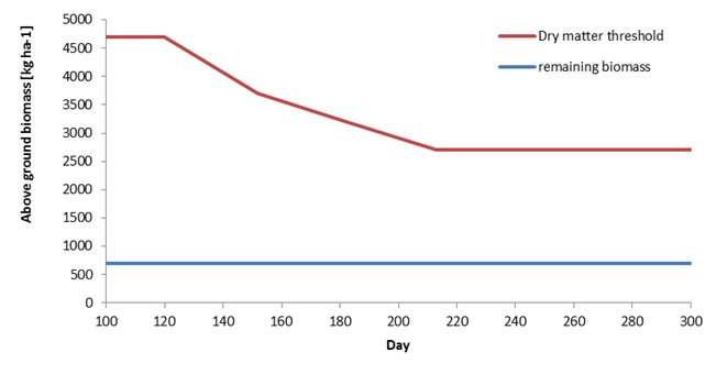
Grassland management also differs substantially from arable crops. Grass can be regularly mowed or grazed by livestock. In SWAP, mowing is initiated either when a minimum threshold of above-ground dry matter is reached or on a specified date. This dry matter threshold may be seasonally variable (Figure 7.8). In addition, mowing schedules can be constrained by imposing a maximum interval between growth periods. To maintain forage quality, mowing should take place within six weeks after the previous event. The amount of above-ground biomass remaining after mowing is defined by the user.
Similary, livestock can enter the field once predefined minimum level of above-ground biomass has been reached. Grazing differs from mowing in that the consumed biomass depends on the grazing days and the livestock density. The user must therefore define the relationship between livestock density, biomass consumption, and dry matter losses due to manure droppings and treading. Additional losses resulting from too wet conditions can also be taken into account.
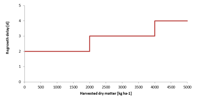
After harvest, the leaf and stem weights are reset according to the partitioning factors. The leaf area index is reset based on the leaf weight. Experiments show that mowing impedes growth for a number of days. This regrowth delay is a function of the dry matter harvest and is part of the input. An example is given in Figure 7.9.
7.5 Root growth
Roots play a key role in the interaction between soil water and crop growth. Accurately estimating root development is therefore essential, as only water and nutrients within the rooted zone are accessible for plant uptake. In SWAP, root development is described through two components: vertical root growth (root extension) and horizontal growth (root distribution). We first present a static approach to simulate root growth, followed by an adaptive approach.
7.5.1 Static root growth
Root extension
Root extension can be simulated in a straightforward way. SWAP offers three methods to calculate the rooting depth:
- Rooting depth as function of development stage
- Daily increase of rooting depth
- Rooting depth as function of above-ground biomass
Rooting depth increases until a maximum is reached and is not affected by stress factors. This maximum depth is determined by crop characteristics or soil constraints. In case of daily increase of rooting depth, root extension proceeds at the maximum daily rate as long as assimilates are available for root growth. Mind that applying static root growth can cause reallocation of root biomass.
Root distribution
With the static approach for root growth, the root distribution is prescribed by the user at the start of the simulation and remains constant over time. In terms of biomass as a function of depth, the root density profile is described by:
\[ w_{j,t+1} = w_{j,t} + g_{j,t} - d_{j,t} \tag{7.39}\]
\[ g_{j,t} = \frac{w_{j,t}}{W_t} + G_t \Delta t \tag{7.40}\]
\[ d_{j,t} = \frac{w_{j,t}}{W_t} + D_t \Delta t \tag{7.41}\]
where \(w_{j,t}\) is the weight of roots (kgdm ha-1) at time \(t\) (d) and soil compartment \(j\), where \(G_t\) and \(D_t\) are respectively the growth and death rate of roots (kgdm ha-1 d-1) during timestep \(\Delta t\) (d), \(g_{j,t}\) and \(d_{j,t}\) are the respective growth and death rates per compartment. From Equation 7.40 and Equation 7.41, it follows that the shape of the root density profile remains constant throughout the growing season.
7.5.2 Adaptive root growth
The adaptive root growth interacts with the soil moisture conditions. For this we implemented a two-step procedure. The first step is to divide the total root growth (\(G\)) into roots assigned to root extension (\(G_\text{ext}\)) and roots that are assigned to the existing rooting depth (\(G_\text{dist}\)).
The amount of roots assigned to the root extension is determined by the relative root density at the bottom of the rootzone \(\left( \frac{w_{n,t}}{(D_{r,t}-z_{top,n,t}} \right)\); kgdm ha-1 cm-1) and the root extension rate \(RR_{ext}\) (cm d-1):
\[ G_{\text{ext},t} = \text{min} \left( G_t \Delta t \frac{w_{n,t}}{(D_{r,t}-z_{top,n,t}} RR_\text{ext} \Delta t\right) \tag{7.42}\]
\[ G_{\text{dist},t} = G_t - G_{\text{ext},t} \tag{7.43}\]
where \(w_{n,t}\) is the weight of roots (kgdm ha-1) at lowest soil compartment (\(n\)).
Root extension
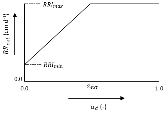
The root extension rate (\(RR_{ext}\)) can either be determined by the maximum daily increase in rooting depth multiplied by the ratio \(T_a/T_p\) or by the transpiration reduction due to drought stress (\(\alpha_d\)), see Figure 7.10 where \(RRI_\text{min}\) and \(RRI_\text{max}\) are respectively the minimum and maximum root extension rate (cm d-1). The maximum root extension rate occurs at \(\alpha_\text{ext}\) (-).
Root distribution
The remaining root growth (\(G_\text{dist}\)) is distributed across existing roots to produce a more adaptive root density profile. This distribution is influenced by the simulated root water extraction from the previous day (\(S_a\)). To account for this interaction Equation 7.40 is extended as follows:
\[ g_{j,t} = \left( 1-f_1\right) \frac{w_{j,t}}{W_t} + G_{\text{dist},t} \Delta t + f_1 \frac{S_{a,j,t}}{S_{a,t}} G_{\text{dist},t} \Delta t \tag{7.44}\]
Here, \(f_1\) is a weighting factor in the range of [0 – 1] that controls how root growth is partitioned between soil compartments. One part is allocated according to the root density profile, while the other is distributed based on root water extraction. If \(S_{a,t}\) = 0, the original formulation in Equation 7.40 is applied.
When root water uptake is simulated using process-based models (see Section 3.5.4), implicit compensation may occur. In such cases, water extraction from a given soil compartment can exceed what would be expected based solely on the local root density. To account for this, Equation 7.44 is reformulated as:
\[ g_{j,t} = \left( 1-f_1\right) \frac{w_{j,t}}{W_t} + G_{\text{dist},t} \Delta t + f_1 \frac{\text{min}\left[T_{a,j,t},T_{p,j,t}\right]}{\sum_{j=1}^n{\text{min}\left[T_{a,j,t},T_{p,j,t}\right]}} G_{\text{dist},t} \Delta t \tag{7.45}\]
where \(T_{p,j,t}\) represents the root length density-weighted potential root water uptake:
\[ T_{p,j} = \frac{L_{\text{rv},j}\Delta z_j}{\sum_{j=1}^nL_{\text{rv},j}\Delta z_j} T_p \tag{7.46}\]
Similar to root growth, decrease in root biomass (Equation 7.41) can be influenced by the simulated reduction of root water extraction, with \(f_2\) as a weight factor:
\[ g_{j,t} = \left( 1-f_2\right) \frac{w_{j,t}}{W_t} + D_t \Delta t + f_2 \frac{\text{max}\left[0,T_{r,j,t}\right]}{\sum_{j=1}^n\text{max}\left[0,T_{r,j,t}\right]} D_t \Delta t \tag{7.47}\]
If \(\sum_{j=1}^n{T_{r,j,t}}\) = 0, the formulation in Equation 7.41 is applied. Under extreme conditions, the above approach may lead to negative values of \(w_{j,t+1}\). To prevent this, a minimum root biomass is enforced in each soil compartment.
All requirements for simulation of an adaptive root density profile are already simulated by either SWAP or WOFOST, except for the parameters \(f_1\) and \(f_2\). Based on rhizobox experiments reported by Maan, Veldhuis, and Wiel (2023), maximum adaptive root growth can be assumed, corresponding to \(f_1\) = \(f_2\) = 1.0.
7.6 CO2 changes
The effect of increasing atmospheric CO2 concentrations can be simulated using input of CO2 concentrations and tables defining the relation between CO2 concentration and maximum assimilation rate \(A_{\text{max}}\), light use efficiency \(\epsilon_{\text{PAR}}\), and potential transpiration rate \(T_{\text{p}}\), respectively. These relations vary per crop and also allow distinction between C3 and C4 crops, see Table 7.1.
In case of static crop growth, the CO2 concentrations only have effect on the potential transpiration.
7.7 User instructions
7.7.1 Crop rotation scheme
Tip 7.1 shows an example of the input for the crop rotation scheme. The switch swcrop controls whether bare soil is simulated or cultivated soil is simulated. For each crop, the user must specify the (maximum) cropping period (CROPSTART and CROPEND), the filename containing the crop input data (CROPFIL), and the type of growth module to be used (CROPTYPE). Information on the simulated crop development is organized according to the user defined output (see Table A.6).
7.7.2 Cropping period
Tip 7.2 shows an example in case the maximum cropping period is influenced by a delay in preparation (SWPREP), sowing (SWSOW) or germination (SWGERM). The timing of harvest (SWHARV) defines the end of the cropping period. Optionally, harvesting can take place before the end of the cropping period if the crop is mature.
7.7.3 Static crop growth
An example of the input file is given in Tip 7.3. Most data are specified as a function of crop development stage, which ranges from 0 to 2. In part 1, the development stage can be defined either linearly in time (specify only duration of crop growth) or based on the temperature sums in the vegetative and reproductive stages.
In part 2, a choice should be made between input of crop factors or crop heights. Crop factors should be used when ETref values are used as input, or when the Penman-Monteith method is used to calculate ETref. Crop heights should be specified if the potential evapotranspiration fluxes are derived directly for the actual crop (see Table 3.2). In that case, also the reflection coefficient and stomatal resistance of the crop should be defined.
In part 3, light extinction coefficients are used to quantify the decrease of solar radiation within a canopy (Chapter 3). Default values of \(\kappa_{\text{dir}} = 0.8\) and \(\kappa_{\text{dif}} = 0.72\) will suffice in most cases.
In part 4, the leaf area during crop development should be specified in order to distribute evapotranspiration fluxes over evaporation and transpiration, as discussed in Chapter 3.
7.7.4 Dynamic crop growth
Input of the detailed crop module has been divided in 9 parts:
- Crop development
- Crop factor of crop height
- Initial values
- Green surface area
- Assimilation
- Conversion of assimilates into biomass
- Maintenance respiration
- Partitioning
- Death rates
An example of the input file is given in Tip 7.4. In general the theorie description in Section 7.4 in combination with the descriptions in the input file will be sufficient to guide the model user. However a few additional remarks should be made here.
In part 2 a choice should be made between input of crop factors or crop heights. Crop factors should be used when ETref values are used as input, or when the Penman-Monteith method is used to calculate ETref. Crop heights should be specified if the potential evapotranspiration fluxes are derived directly for the actual crop (see Table 3.2). In that case also the reflection coefficient and stomatal resistance of the crop should be defined.
In part 8 the user should specify the partitioning factors as function of crop development stage. As explained in Section 7.4.7, WOFOST first divides the gross dry matter among roots and shoots (leafs, stems and storage organs together), using the partitioning factor for roots. Next WOFOST divides the gross dry matter directed to the shoots among leafs, stems and storage organs, using the partitioning factors for these plant organs. At any development stage the sum \(\xi\)leaf + \(\xi\)stem + \(\xi\)stor must equal one.
Boons-Prins et al. (1993) documented specific parameters for the crops winter wheat, grain maize, spring barley, rice, sugar beet, potato, field bean, soy bean, winter oilseed rape and sunflower. WOFOST input files for some crops will be provided with the SWAP program.
For the simulation of grassland some adaptations in WOFOST have been made. Tip 7.5 shows the input data for the initialisation of grass growth.
Tip 7.6 shows the management section of dynamic grass growth. Mowing or grazing (with dewooling) is initiated either when a minimum threshold of above-ground dry matter is reached or on a specified date (SWHARVEST). The matter threshold is set by DMGRZTB and DMMOWTB for grazing and mowing, respectively. In addition, a maximum interval between growth periods can be considered (MXGDGRZ and MXGDMOW). The amount of above-ground biomass remaining after grazing (with dewooling) of mowing is defined by DMRESTGRZ, DMRESTDEW and DMRESTMOW.
When grazing occurs, the amount of biomass consumed is determined by the number of grazing days (DAYGRZ), the daily dry matter uptake (UPTGRZ) and dry matter losses caused by manure droppings and treading (LOSSGRZ). Additional losses due to excessively wet conditions can also be considered (SWLOSSGRZZ and SWLOSSMOW), expressed as a function of pressure head at a given depth.
7.7.5 Root growth
The simulation of root extension is governed by SWRD. When the root extension is modelled as a daily increase, the maximum extension rate can be reduced based on the ratio of actual to potential transpiration (SWDMI2RD = 1), or adjusted according to drought stress (SWDMI2RD = 2).
The initial relative root length density distribution (RDCTB) is used by SWAP to determine the distribution of potential root water uptake rates. By default, this relative root distribution remains constant throughout the cropping period. When SWRDC = 1, the relative root distribution is modified based on the simulated root water extraction.
When root water uptake is modelled with detailed oxygen or drought stress, the specific root lenght (LRV) and root radius (ROOTRADIUS) must be provided in the input file.
7.7.6 Stress factors
The input of stress factors is presented in Tip 7.8 and is divided into four parts:
- Drought stress
- Oxygen stress
- Salinity stress
- Compensation of root water uptake stress
For drought stress (Part 1) the user should choose between the simple reduction function of Feddes et al. (1978), or the more process based reduction function of De Jong van Lier et al. (2013) or De Willigen et al. (2012). Appendix G provides the critical pressure head values for drought stress according to Feddes et al. (1978), based on Taylor and Ashcroft (1972).
For oxygen stress (Part 2), the available options include the simple reduction function of Feddes et al. (1978) and the more process-based reduction approach described by Bartholomeus et al. (2008).
Part 3 defines the parameters describing the reduction in root water uptake as function of salinity concentrations, following Maas and Hoffman (1977). Parameters values for the Maas and Hoffman reduction function are available for many crops (Maas 1990). Appendix K list the input parameters SALTMAX and SALTSLOPE for a range of crops.
In Part 4, the original Feddes reduction function can be extended with compensation according to Jarvis (1989) by specifying a value for ALPHACRIT. This parameter represents the relative transpiration level up to which reduction in root water uptake are compensated. Compensation according to Jarvis (1989) cannot be combined with the approaches of De Jong van Lier et al. (2013) and De Willigen et al. (2012), since implicit compensation is already incorporated in these concepts.
7.7.7 CO2 changes
Tip 7.9 presents the input data describing changes in CO2 and their effect on the maximum assimilation rate (CO2AMAXTB), light use efficiency (CO2EFFTB), and potential transpiration rate (CO2TRATB). Yearly CO2 concentrations can be supplied in the *.crp file (CO2YEAR and CO2PPM) or a separate input file (ATMOFIL).
7.7.8 Rainfall interception
Tip 7.10 shows the interception input data. For agricultural crops, just one interception coefficient cofab for the Von Hoyningen-Hune and Braden concept is required. The default value of cofab = 0.25 cm will suffice for most agricultural crops in case of daily rainfall (SWRAIN = 0). In the case of forests (Gash concept), SWAP requires coefficients for free throughfall and stem flow, canopy storage capacity, and average rainfall and evaporation fluxes as a function of crop development. The specified average rainfall and evaporation flux values are independent of other input weather data. In case of detailed rainfall records the usage of Hoyningen-Braden and Gash cannot be used. Instead interception can be simulated by Rutter where we assume evaporation from a canopy reservoir (SWINTER = 3).