9  Soil temperature

9.1 Introduction

Soil temperature affects many physical, chemical, and biological processes in the topsoil, for instance the surface energy balance, soil hydraulic properties, decomposition rate of solutes, and growth rate of roots. Currently, SWAP uses soil temperature in the following processes:

• Suppression of grass growth due to low temperatures
• Reduction of hydraulic conductivity and root water uptake at low temperatures
• Mineralization rate
• Respiration rate (and some other oxygen-related processes)
• Solute decomposition rate

Other temperature relations can be easily included if needed. SWAP calculates the soil temperatures either analytically or numerically. In the following sections, the heat flow equations and the applied analytical and numerical solutions are discussed.

9.2 Temperature conductance equation

If we consider heat transport only by convection, the one-dimensional soil heat flux, \(q_{\text{heat}}\) (J cm^-2 d^-1), can be described as:

\[ q_{\text{heat}} = -\lambda_{\text{heat}} \frac{\partial T}{\partial z} \tag{9.1}\]

where \(\lambda_{\text{heat}}\) is the thermal conductivity (J cm^-1 °C^-1 d^-1) and \(T\) is the soil temperature (°C).

Conservation of energy results in:

\[ C_{\text{heat}} \frac{\partial T}{\partial t} = -\frac{\partial q_{\text{heat}}}{\partial z} \tag{9.2}\]

where \(C_{\text{heat}}\) is the soil heat capacity (J cm^-3 °C^-1).

Combination of Equation 9.1 and Equation 9.2 yields the differential equation for soil heat flow:

\[ C_{\text{heat}} \frac{\partial T}{\partial t} = \frac{\partial (\lambda_{\text{heat}} \frac{\partial T}{\partial z})}{\partial z} \tag{9.3}\]

In general, in the liquid phase, radiation and convection will also transport heat. As the contribution of radiation and convection to soil heat transport in general is small compared to conductance (Moene and Dam 2014), SWAP only considers conductance. In the vapor phase, diffusion may contribute to soil heat transport. The rate of heat transfer by water vapor diffusion is small and proportional to the temperature gradient (De Vries 1975). Therefore, such diffusion can be taken into account by slightly increasing the soil thermal diffusivity. This approach is followed in SWAP as well. Apparent thermal properties rather than real thermal properties are assumed to account for both conductive and non-conductive heat flow.

9.3 Numerical solution

The parameters \(\lambda_{\text{heat}}\) and \(C_{\text{heat}}\) strongly depend on the soil moisture content. Therefore, in general Equation 9.3 can only be solved with a numerical solution. SWAP employs a fully implicit finite difference numerical scheme to solve Equation 9.3:

\[ C_i^{j+1} (T_i^{j+1} - T_i^j) = \frac{\Delta t^j}{\Delta z_i} \left[ \lambda_{i-1/2}^{j+1/2} \frac{T_{i-1}^{j+1} - T_i^{j+1}}{\Delta z_u} - \lambda_{i+1/2}^{j+1/2} \frac{T_i^{j+1} - T_{i+1}^{j+1}}{\Delta z_l} \right] \tag{9.4}\]

where superscript \(j\) denotes the time level, subscript \(i\) is the node number, \(\Delta z_u = z_{i-1} - z_i\) and \(\Delta z_l = z_i - z_{i+1}\). As the coefficients \(C_{\text{heat}}\) and \(\lambda_{\text{heat}}\) are not affected by the soil temperature itself, Equation 9.4 is a linear equation.

Both \(C_{\text{heat}}\) and \(\lambda_{\text{heat}}\) depend on the soil composition. The volumetric heat capacity is calculated as a weighted mean of the heat capacities of the individual components [De_Vries_1963]:

\[ C_{\text{heat}} = f_{\text{sand}} C_{\text{sand}} + f_{\text{clay}} C_{\text{clay}} + f_{\text{organic}} C_{\text{organic}} + \theta C_{\text{water}} + f_{\text{air}} C_{\text{air}} \tag{9.5}\]

where \(f\) and \(C\) on the right-hand side of Equation 9.5 are the volume fraction (cm³ cm^-3) and volumetric heat capacity (J cm^-3 °C^-1) of each component, respectively, and the components are indicated in the subscripts. Table 9.1 gives values of \(C\) for the different soil components.

Table 9.1: Volumetric heat capacity and thermal conductivity of the soil components.

Component	Volumetric heat capacity Cheat (J cm -3 °C-1)	Thermal conductivity λheat (J cm -1 °C-1 d-1)
Sand	2.128000	7603
Clay	2.385000	2523
Organic	2.496000	216
Water	4.180000	492
Air (°C)	0.001212	variable

In order to calculate \(C_{\text{heat}}\) from Equation 9.5, the percentage (by volume) of sand and clay, denoted \(VP_{\text{sand}}\) and \(VP_{\text{clay}}\), respectively, must be specified by the SWAP user. \(VP_{\text{sand}}\) and \(VP_{\text{clay}}\) should be provided as percentages of the total solid soil matter and may differ for each soil layer. The total volume fraction of solid matter is given by:

\[ \theta_{\text{solid}} = 1 - \theta_{\text{sat}} \tag{9.6}\]

where \(\theta_{\text{sat}}\) is the saturated volumetric water content. The volume fraction of air is equal to the saturated minus the actual water content:

\[ f_{\text{air}} = \theta_{\text{sat}} - \theta \tag{9.7}\]

\(f_{\text{sand}}\), \(f_{\text{clay}}\), and \(f_{\text{organic}}\) are then calculated by:

\[ f_{\text{sand}} = \frac{VP_{\text{sand}}}{100} \theta_{\text{solid}} \tag{9.8}\]

\[ f_{\text{clay}} = \frac{VP_{\text{clay}}}{100} \theta_{\text{solid}} \tag{9.9}\]

\[ f_{\text{organic}} = \theta_{\text{solid}} - f_{\text{sand}} - f_{\text{clay}} \tag{9.10}\]

where it has been assumed that solid matter that is not sand or clay, is organic.

Table 9.1 also lists the thermal conductivities, which are largest for sand and clay, an order smaller for organic material and water, and again an order smaller for air. Hence the space-average thermal conductivity of a soil depends upon its mineral composition and organic matter content, as well as the volume fractions of water and air. Since the thermal conductivity of air is much smaller than that of water or solid matter, a high air content (or low water content) corresponds to a low thermal conductivity.

The components that affect \(\lambda_{\text{heat}}\) are the same as those affecting \(C_{\text{heat}}\). However, the variation in \(\lambda_{\text{heat}}\) is much greater than the variation of \(C_{\text{heat}}\). In the range of soil wetness normally experienced in the field, \(C_{\text{heat}}\) may undergo a threefold or fourfold change, whereas the corresponding change in \(\lambda_{\text{heat}}\) may be hundredfold or more. Unlike heat capacity, thermal conductivity is also sensitive to the sizes, shapes, and spatial arrangements of the soil particles (Hillel 1980).

The thermal conductivity is found by considering the soil as a continuous liquid or gaseous phase in which soil and respectively gas or liquid ‘particles’ are dispersed. In the case of a ‘wet’ soil (\(\theta > \theta_{\text{wet}}\)) liquid water is assumed to be the continuous phase and the thermal conductivity is given by:

\[ \lambda_{\text{heat}} = \frac{x_{\text{s-w}} f_{\text{s}} \lambda_{\text{s}} + x_{\text{c-w}} f_{\text{c}} \lambda_{\text{c}} + x_{\text{o-w}} f_{\text{o}} \lambda_{\text{o}} + x_{\text{w-w}} \theta \lambda_{\text{w}} + x_{\text{a-w}} f_{\text{a}} \lambda_{\text{a}}}{x_{\text{s-w}} f_{\text{s}} + x_{\text{c-w}} f_{\text{c}} + x_{\text{o-w}} f_{\text{o}} + x_{\text{w-w}} \theta + x_{\text{a-w}} f_{\text{a}}} \tag{9.11}\]

where the subscripts a, c, o, s and w refer to air, clay, organic, sand and water, respectively. The \(\lambda\)–values on the right-hand side of Equation 9.11 refer to the thermal conductivities (J cm^-1 °C^-1 d^-1) of each individual component, as listed in Table 9.1. The weighting factors \(x_{\text{mn}}\) for component \(m\) particles suspended in the continuous phase \(n\) depend on the ratio of the specific thermal conductivities of component \(m\) and \(n\) and on the shape of \(m\) particles in the direction of the temperature gradient. When we assume the particles to be spheroids whose axes are randomly oriented in the soil (Ten Berge 1986), the weighting factors can be calculated by:

\[ x_{\text{mn}} = \frac{0.66}{1 + g_m \left(\frac{\lambda_m}{\lambda_n} - 1\right)} + \frac{0.33}{1 + \left(\frac{\lambda_m}{\lambda_n} - 1\right)(1 - 2g_m)} \tag{9.12}\]

The shape factors and weights calculated using Equation 9.12 are given in Table 9.2. The thermal conductivity is quite sensitive to the air shape factor (\(g_a\)), which appears to depend on the air content itself and is calculated as:

\[ g_a = \begin{cases} 0.333 - \frac{\theta_{\text{sat}} - \theta}{\theta_{\text{sat}}} (0.333 - 0.035) & \text{for wet soils} \space \theta > \theta_{\text{wet}}\\ 0.013 + \frac{\theta}{\theta_{\text{dry}}} (g_{\text{a,dry}} - 0.013) & \text{for dry soils} \space \theta < \theta_{\text{dry}} \end{cases} \tag{9.13}\]

where \(g_{\text{a,dry}}\) is the value at \(\theta = \theta_{\text{dry}}\). In this way \(g_a\) varies between 0.013 (\(\theta = 0\)) and 0.333 (\(\theta = \theta_{\text{sat}}\)).

For ‘dry’ soil (\(\theta < \theta_{\text{dry}}\)), air is considered as the continuous phase and the conductivity is given by:

\[ \lambda_{\text{heat}} = \frac{1.25 (x_{\text{s-a}} f_{\text{s}} \lambda_{\text{s}} + x_{\text{c-a}} f_{\text{c}} \lambda_{\text{c}} + x_{\text{o-a}} f_{\text{o}} \lambda_{\text{o}} + x_{\text{w-a}} \theta \lambda_{\text{w}} + x_{\text{a-a}} f_{\text{a}} \lambda_{\text{a}})}{x_{\text{s-a}} f_{\text{s}} + x_{\text{c-a}} f_{\text{c}} + x_{\text{o-a}} f_{\text{o}} + x_{\text{w-a}} \theta + x_{\text{a-a}} f_{\text{a}}} \tag{9.14}\]

which is similar to Equation 9.11 with an empirical correction factor (Ten Berge 1986).

In the case that neither water nor air can be considered as the continuous phase (\(\theta_{\text{dry}} < \theta < \theta_{\text{wet}}\)), \(\lambda_{\text{heat}}\) is found by interpolation between values at the wet and dry limits:

\[ \lambda_{\text{heat}} (\theta) = \lambda_{\text{heat}} (\theta_{\text{dry}}) + \left(\frac{\lambda_{\text{heat}} (\theta_{\text{wet}}) - \lambda_{\text{heat}} (\theta_{\text{dry}})}{\theta_{\text{wet}} - \theta_{\text{dry}}}\right) (\theta - \theta_{\text{dry}}) \tag{9.15}\]

The values of \(\theta_{\text{dry}}\) and \(\theta_{\text{wet}}\) are taken as 0.02 and 0.05 cm³ cm^-3, respectively. We refer to De Vries (1975), Ten Berge (1986), and Moene and Dam (2014) for more information on the calculation of \(\lambda_{\text{heat}}\).

Table 9.2: Shape and weight factors for different components in water and air phases, as used for thermal conductivity calculations (Ashby et al. 1996).

	Sand	Clay	Organic	Water	Air
Shape factor (g)	0.1400	0.1250	0.5000	0.1400	Equation 9.13
Weight factor (xwater) for water as continuous phase	0.2461	0.7317	1.2602	1.0000	1.6062
Weight factor (xair) for air as continuous phase	0.0143	0.6695	0.4545	0.1812	1

At the soil surface, either the daily average air temperature \(T_{\text{avg}}\) or measured soil surface temperatures can be used as a boundary condition. In the case of a snow layer and the use of \(T_{\text{avg}}\), SWAP will adjust \(T_{\text{avg}}\) as described in Chapter 10. At the bottom of the soil profile, either soil temperatures can be specified or \(q_{\text{heat}} = 0.0\) can be selected. The latter option is valid for large soil columns.

Application of Equation 9.4 to each node and including the boundary conditions at the top and bottom of the soil profile results in a tri-diagonal system of equations, as shown in Appendix L. SWAP solves the equations with LU-decomposition for tridiagonal systems (Press et al. 1989).

9.4 Analytical solution

If the values of \(\lambda_{\text{heat}}\) and \(C_{\text{heat}}\) are considered to be constant within the discretized soil layer and time interval, the soil thermal diffusivity \(D_{\text{heat}}\) (cm² d^-1) can be defined as:

\[ D_{\text{heat}} = \frac{\lambda_{\text{heat}}}{C_{\text{heat}}} \tag{9.16}\]

and Equation 9.3 simplifies to:

\[ \frac{\partial T}{\partial t} = D_{\text{heat}} \frac{\partial^2 T}{\partial z^2} \tag{9.17}\]

This partial differential equation can be solved for simple boundary conditions, assuming \(D_{\text{heat}}\) constant or very simple functions for \(D_{\text{heat}}\) (Van Wijk 1966; Feddes 1971; Wesseling 1987). A commonly used top boundary condition is a sinusoidally varying soil surface temperature:

\[ T(0, t) = T_{\text{mean}} + T_{\text{ampl}} \sin \left( \frac{1}{2}\pi + \omega(t - t_{\text{max}}) \right) \tag{9.18}\]

where \(T_{\text{mean}}\) is the mean yearly temperature (°C), \(T_{\text{ampl}}\) is the wave amplitude (°C), \(\omega = 2\pi / \tau\) is the angular frequency, where \(\tau\) is the period of the wave (d), \(t\) is time (d) starting January 1st and \(t_{\text{max}}\) equals \(t\) when the temperature reaches its maximum. In case of a semi-infinite soil profile with constant \(D_{\text{heat}}\) and using Equation 9.18, the solution to Equation 9.17 is:

\[ T(z, t) = T_{\text{mean}} + T_{\text{ampl}} e^{\frac{z}{d_{\text{temp}}}} \sin \left( \frac{1}{2}\pi + \omega(t - t_{\text{max}}) + \frac{z}{d_{\text{temp}}} \right) \tag{9.19}\]

where \(d_{\text{temp}}\) is the damping depth (cm), which equals:

\[ d_{\text{temp}} = \sqrt{\frac{2D_{\text{heat}}}{\omega}} \tag{9.20}\]

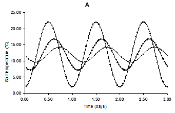
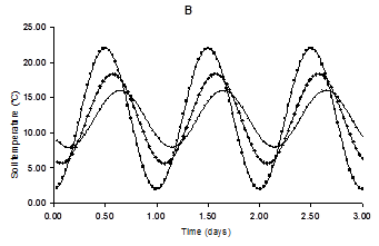
Equation 9.19 can be used for daily or yearly fluctuations. Measured values of \(D_{\text{heat}}\) for various dry and wet soils are given in Table 9.3. Figure 9.1 gives an example of calculated soil temperatures for a dry and wet sand soil. The sinusoidal temperature fluctuations at each depth are reduced in amplitude and delayed in time with respect to the top boundary condition. Although the heat capacity of wet sand is higher than of dry sand, the temperature wave in the wet sand is less attenuated due to the higher thermal conductivity.

Table 9.3: Thermal diffusivity \(D_\text{heat}\) (cm² d^-1) for various dry and wet soils (Jury et al. 1991).

Soil type	Dry	Wet
Sand	147	380
Loam	156	518
Clay	156	320
Peat	112	104

(a)

(b)

Figure 9.1: Calculated soil temperatures at depths z = 0, z = -5 and z = -10 cm for a dry (A) and a wet (B) sand soil. The following input data were used: \(T_{\text{mean}}\) = 12 °C, \(T_{\text{ampl}}\) = 10 °C, \(\tau\) = 1 d, \(t_{\text{max}}\) = 0.5 d and \(D_{\text{heat}}\) = 147 (dry) and 380 (wet) cm² d^-1.

9.5 User instructions

Tip 9.1 lists the input data for heat transport. When the analytical method is used, the parameters describing the soil surface temperature wave and the demping depth should be specified. The damping depth might be derived from Equation 9.20 and the thermal diffusivity values from Table 9.3. When the numerical method is used, information should be given of the soil texture, initial soil temperatures and type of bottom boundary condition.

In case top soil temperatures are provided in a separate file (swtophea = 2), the file tsoilfile must have the extension *.tss. The files should contain two data columns: the first column (with header DATET) contains the date (yyyy-mm-dd), and the second column (header TTOP) contains the soil surface temperature (°C).

Tip 9.1: Information on heat transport in main file *.swp

**********************************************************************************

*** HEAT FLOW SECTION ***

**********************************************************************************

* Switch for simulation of heat transport:
  SWHEA = 1                  ! 0 = No simulation of heat transport
                             ! 1 = Simulation of heat transport

* Switch for calculation method:
  SWCALT = 2                 ! 1 = Analytical method
                             ! 2 = Numerical method

* In case of the analytical method (SWCALT=1) specify:
* If SWCALT=1 specify the following heat parameters:
  TAMPLI = 10.0              ! Amplitude of annual temperature wave at soil surface [0..50 degree C, R]
  TMEAN = 15.0               ! Mean annual temperature at soil surface [-10..30 degree C, R]
  TIMREF = 90.0              ! Time at which the sinus temperature wave reaches its top [0..366.0 d, R]
  DDAMP = 50.0               ! Damping depth of soil temperature wave [1..500 cm, R]

* In case of the numerical method (SWCALT=2) specify:
* Specify for each physical soil layer the soil texture (g/g mineral parts) and the organic matter content (g/g dry soil):

 PSAND PSILT PCLAY ORGMAT
   0.8  0.15  0.05    0.1
   0.8  0.15  0.05    0.1
* End of table

* If SWINCO=1 or SWINCO=2, specify initial temperature [-50..50 degree C, R] as function of soil depth [-100000..0 cm, R]:

  TSOILTB =
 -10.0 15.0
 -40.0 12.0
 -70.0 10.0
 -95.0  9.0
* End of table

* Define top boundary condition: 
  SWTOPBHEA = 1              ! 1 = Use air temperature of meteo input file as top boundary
                             ! 2 = Use measured top soil temperature as top boundary

* If SWTOPBHEA=2, specify name of input file with soil surface temperatures
  TSOILFILE = 'swap'         ! File name without extension .TSS [A16]

* Define bottom boundary condition:
  SWBOTBHEA = 1              ! 1 = No heat flux
                             ! 2 = Prescribe bottom temperature

* If SWBOTBHEA=2, specify bottom boundary temperature TBOT [-50..50 degree C, R] as function of date DATET [YYYY-MM-DD]:

      DATET  TBOT
 2002-01-01 -15.0
 2002-06-30 -20.0
 2002-12-23 -10.0
* End of table

**********************************************************************************

Ashby, M., A. J. Dolman, P. Kabat, E. J. Moors, and M. J. Ogink-Hendriks. 1996. SWAPS Version 1.0. Technical Reference Manual. Book. Technical Document 42, Winand Staring Centre, Wageningen, The Netherlands.

De Vries, D. A. 1975. “Heat Transfer in Soils.” Book Section to Heat and Mass Transfer in the Biosphere. I. Transfer Processes in Plant Environment, edited by D. A. De Vries and N. H. Afgan. Scripts Book Company, Washington D.C.

Feddes, R. A. 1971. Water, Heat and Crop Growth. PhD Thesis. Book. Wageningen Agricultural University, The Netherlands.

Hillel, D. 1980. Fundamentals of Soil Physics. Book. Academic Press, San Diego, CA.

Jury, W. A., W. R. Gardner, and W. H. Gardner. 1991. Soil Physics. Fifth Edition. Book. Wiley, New York.

Moene, A. F., and J. C. van Dam. 2014. Transport in the Atmosphere-Vegetation-Soil Continuum. Book. Cambridge University Press. https://doi.org/10.1016/j.apradiso.2013.12.019.

Press, W. H., B. P. Flannery, S. A. Teukolsky, and W. T. Vetterling. 1989. Numerical Recipes. The Art of Scientific Computing. Book. Cambridge University Press.

Ten Berge, H. F. M. 1986. Heat and Water Transfer at the Bare Soil Surface: Aspects Affecting Thermal Images. PhD Thesis. Book. Wageningen Agricultural University, Wageningen, The Netherlands.

Van Wijk, W. R. 1966. Physics of Plant Environment. Second Edition. Book. North Holland Publ. Comp., Amsterdam, The Netherlands.

Wesseling, J. G. 1987. “Invloed van Bodemsoort En Vochtgehalte Op de Bodemtemperatuur. Een Theoretische Beschouwing.” Journal Article. Cultuurtechnisch Tijdschrift 27: 117–28.