| Description of uniform surface | ETp | rs (s m-1) | hcrop (cm) | αr (-) |
|---|---|---|---|---|
| Wet canopy, completely covering the soil | ETw0 | input | input | input |
| Dry canopy, completely covering the soil | ETp0 | input | input | input |
| Wet, bare soil | Ep0 | 0.0 | 0.1 | 0.15 |
3 Evapotranspiration and rainfall interception
3.1 Introduction
In contrast to rainfall, accurate measurement of evapotranspiration fluxes is far from trivial. Evapotranspiration fluxes strongly vary with the local hydrological conditions. Therefore, SWAP simulates evapotranspiration fluxes employing basic weather data or reference crop evapotranspiration data, as discussed in this chapter.
Rainfall and irrigation minus the sum of transpiration, evaporation, and interception determine the amount of infiltration in the soil (Figure 3.1) and groundwater fluxes. In general, the sums of rainfall+irrigation and transpiration+evaporation+interception are large compared to their difference, which equals the infiltration. This means that relative errors in these sums will magnify in relative errors of infiltration and groundwater fluxes. Therefore, reliable soil water and groundwater fluxes require accurate simulation of evapotranspiration and interception fluxes.
In general, the daily water fluxes passing through a canopy are large compared to the amounts of water stored in the canopy itself. Therefore, we will assume that root water extraction in the soil is equal to plant transpiration. While root water extraction may occur throughout the root zone, soil evaporation occurs at the interface soil-atmosphere. The consequence is that during drying conditions, evaporation fluxes decline much more rapidly than transpiration fluxes. Water harvesting, by leaving fields fallow during one or several seasons, uses this phenomenon. Because of the different physical behaviour of transpiration and evaporation, SWAP will consider evaporation and transpiration separately.
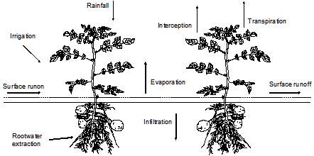
In this chapter, we will first discuss the rainfall interception as used for low vegetation and forests. Next, we describe the simulation of potential evapotranspiration and its distribution into potential transpiration and evaporation for partly covered soils. Then, we will discuss the reduction of transpiration for wet, dry, and saline soil conditions, and the reduction of evaporation for dry top soils. In the last part, the related model input is described.
3.2 Rainfall interception
Three methods are available in SWAP to simulate rainfall interception. The methods Hoyningen-Braden for agricultural crops and Gash for forests use daily rainfall amounts only. In case of detailed rainfall records (< 1 day) the method Rutter can be used. In case irrigation water is applied with sprinklers, SWAP will simulate separately interception of rainfall and irrigation. This is required because the solute concentration of both water sources may be different. Observed rainfall Pgross minus intercepted rainfall \(P_i\) is called net rainfall \(P_\text{net}\). Likewise, applied irrigation depth \(I_\text{gross}\) minus intercepted irrigation water is called net irrigation depth \(I_\text{net}\).
3.2.1 Method Hoyningen-Braden
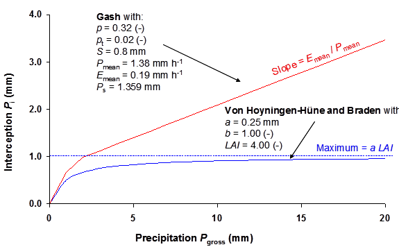
For agricultural crops and for pasture Von Hoyningen-Hüne (1983) and Braden (1985) proposed the following general formula for canopy interception (Figure 3.2):
\[ P_i = a LAI \left(1 - \frac{1}{1 + \left(\frac{V_\text{c} P_\text{gross}}{a LAI}\right)}\right) = \frac {a LAI V_\text{c} P_\text{gross}} {a LAI + V_\text{c} P_\text{gross}} \tag{3.1}\]
where \(P_i\) is intercepted precipitation cm d-1, \(LAI\) is leaf area index, \(P_{\text{gross}}\) is gross precipitation cm d-1, \(a\) is an empirical coefficient cm d-1 and \(V_\text{c}\) represents the soil cover fraction (-). For increasing amounts of precipitation, the amount of intercepted precipitation asymptotically reaches the saturation amount \(aLAI\). In principle, \(a\) must be determined experimentally and should be specified in the input file. In case of ordinary agricultural crops, we may assume \(a\) = 0.025 cm d-1.
The vegetation cover is based on solar light extinction within the canopy. The most common method assumes that the net radiation inside the canopy decreases according to an exponential function (Goudriaan 1977; Belmans, Wesseling, and Feddes 1983) according to:
\[ V_\text{c} = 1 - e^{-\kappa_\text{gr} LAI} \tag{3.2}\]
where \(\kappa_\text{gr}\) (-) is the extinction coefficient for solar radiation and \(LAI\) is the actual leaf area index (-). Ritchie (1972) and Feddes, Kowalik, and Zaradny (1978) used \(\kappa_\text{gr}\) = 0.39 for common crops. More recent approaches estimate \(\kappa_\text{gr}\) as the product of the extinction coefficient for diffuse visible light, \(\kappa_\text{dif}\) (-), which varies with crop type from 0.4 to 1.1, and the extinction coefficient for direct visible light, \(\kappa_\text{dir}\) (-):
\[ \kappa_\text{gr} = \kappa_\text{dir} \kappa_\text{dif} \tag{3.3}\]
The method of Von Hoyningen-Hüne and Braden is based on daily precipitation values. Although a rainfall duration may be specified , the interception will be based on daily amounts.
3.2.2 Method Gash
A main drawback of the method of Von Hoyningen-Hüne and Braden is that the effect of rain duration and evaporation during the rain event is not accounted for. In case of trees and forests, evaporation of intercepted water during rainfall cannot be neglected. Gash (1979; 1995) formulated a physically based and widely used interception formula for forests. He considered rainfall to occur as a series of discrete events, each comprising a period of wetting up, a period of saturation, and a period of drying out after the rainfall. The canopy is assumed to have sufficient time to dry out between storms. During wetting up, the increase of intercepted amount is described by:
\[ \frac{\partial P_\text{i}}{\partial t} = c P_\text{mean} - \frac{P_\text{i}}{S_\text{c}} E_\text{c,mean} \tag{3.4}\]
where \(P_{\text{mean}}\) is the mean rainfall rate (mm h-1), \(E_{\text{c,mean}}\) is the mean evaporation rate of intercepted water when the canopy is saturated (mm h-1 per unit area of cover), \(S_\text{c}\) is the maximum storage of intercepted water in the canopy (mm per unit area of cover), and \(c\) is the canopy cover (-).
The fraction of canopy cover depends on the stemflow and the throughfall:
\[ c = 1 - p - p_\text{t} \tag{3.5}\]
where \(p\) is a free throughfall coefficient (-) and \(p_\text{t}\) is the proportion of rainfall diverted to stem flow (-).
Integration of Equation 3.4 yields the amount of rainfall which saturates the canopy, \(P_s\) (mm):
\[ P_\text{s} = -\frac{P_\text{mean} S_\text{c}} {E_\text{c,mean}} \ln\left(1-\frac{E_\text{c,mean}}{P_\text{mean}} \right) \quad \text{with} \quad 1-\frac{E_\text{c,mean}}{P_\text{mean} } \ge 0 \tag{3.6}\]
For small storms (\(P_\text{gross} < P_\text{s}\)) the interception can be calculated from:
\[ P_\text{i} = c P_\text{gross} \tag{3.7}\]
For large storms (\(P_\text{gross} > P_\text{s}\)) the interception according to Gash (1979) follows from:
\[ P_\text{i} = c \left ( P_s + \frac{c E_\text{c,mean}}{P_\text{mean}} (P_\text{gross} - P_\text{s}) \right ) \tag{3.8}\]
The relation of Gash for typical values of a pine forest as a function of rainfall amounts is illustrated in Figure 3.2. The slope \(\partial P_\text{i} / \partial P_\text{gross}\) before saturation of the canopy equals \(c\), after saturation of the canopy this slope equals \(E_\text{c,mean} / P_\text{mean}\).
SWAP uses mean intensities of rainfall and evaporation rate to calculate the amount of rainfall which saturates the canopy, according to Equation 3.6. Next, depending on the total amount of rainfall during a day, the amount of interception is calculated according to either Equation 3.7 or Equation 3.8.
3.2.3 Method Rutter
In case of detailed rainfall records the usage of Hoyningen-Braden and Gash cannot be used. Instead interception can be simulated by Rutter where we assume evaporation from a canopy reservoir.
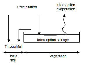
The used modelling method is a simplified version of the approach presented by (Valente, David, and Gash 1997) for tree vegetation, which in turn is an adaptation of (Rutter et al. 1971). In the approach presented here the canopy and trunk reservoirs are lumped together; a second modification involves the canopy evaporation rate which is assumed to be equal to the evaporation rate of a wet canopy instead of depending on the degree of canopy saturation.
The Rutter interception is calculated per time step. The change during a time step of the amount of rainfall stored in the canopy reservoir is described by:
\[ S_{t+1} = S_{t0} + V_\text{c} \left ( P_\text{g} - E_\text{i} \right ) \Delta t \tag{3.9}\]
Where \(S\) is the water stored in canopy reservoir (cm), \(V_\text{c}\) is the soil cover fraction (see above), \(P_\text{g}\) gross precipitation rate (cm d-1) and \(E_\text{i}\) evaporation rate from a wet canopy (cm d-1). Of course, the canopy has a maximum storage capacity and the storage cannot become less than zero. The canopy reservoir has a maximum storage capacity that is related to the leaf area and therefore depends on the season:
\[ S_\text{max} = S_\text{lai} LAI \tag{3.10}\]
Where \(S_\text{max}\) is the maximum storage capacity of the canopy reservoir (cm) and \(S_\text{lai}\) is the storage capacity per unit of leaf area index (cm LAI-1). When the canopy reservoir has reached the maximum storage capacity all excess precipitation (precipitation minus canopy evaporation) becomes throughfall.
When the canopy reservoir is empty, and the rainfall rate is less than the evaporation rate, then all the rainfall on the canopy will evaporate (\(V_\text{c} P_\text{g} \Delta t\)).
The intercepted rainfall can consist of an evaporation from the interception reservoir and the increase of water stored in the canopy reservoir. The net precipitation can, therefore, be described by: \[ P_\text{net} = \begin{cases} \left (1 - V_\text{c} \right ) P_\text{g} - V_\text{c} E_\text{i} & S_\text{t} < S_\text{max} \\ P_\text{g} - V_\text{c} E_\text{i} & S_\text{t} = S_\text{max} \text{ and } P_\text{g} \ge 0 \end{cases} \tag{3.11}\]
3.3 Potential evapotranspiration of uniform surfaces
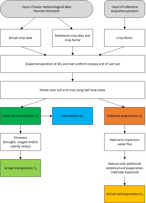
Evapotranspiration refers to 4 processes: transpiration of the plants, evaporation of the soil, evaporation of water intercepted by vegetation and evaporation of water ponding on the soil surface. The addition ‘potential’ refers to non-limiting soil conditions. The potential evapotranspiration flux is therefore only determined by atmospheric conditions and plant characteristics. In SWAP, we assume the atmospheric conditions to be external conditions, which are representative of the area for which the simulations are performed. Starting point in the calculations is the determination of the potential evapotranspiration of different uniform surfaces. The model offers two methods to calculate this potential evapotranspiration (Figure 3.4): the Penman-Monteith method and the reference evapotranspiration method. Both methods can be combined with crop factors; Penman-Monteith can also be applied without crop factors.
By default, evapotranspiration is distributed uniformly over the day. Diurnal variations in evapotranspiration can be represented by distributing the evapotranspiration according to a sine wave over the photoperiod (daylight hours). If a more detailed representation of the diurnal variation is required, the Penman-Monteith equation can be applied using shorter time intervals.
3.3.1 Penman Monteith method
Elaborating the physical theory of Penman (1948), Monteith (1965) derived an equation that describes the evapotranspiration from a dry, uniform, vegetated surface, which is optimally supplied with water. This equation is known as the Penman-Monteith equation. Jensen, Burman, and Allen (1990) analysed the performance of 20 different evapotranspiration formulas using lysimeter data of 11 stations around the world under different climatic conditions. The Penman-Monteith formula ranked as the best for all climatic conditions. Therefore this equation has become an international standard for the calculation of potential evapotranspiration (Allen et al. 1998), and is applied in SWAP.
For a closed canopy with insignificant evaporation from the soil, the Penman-Monteith equation can be written as (Monteith 1965, 1981):
\[ ET_\text{p} = \frac {\frac{\Delta_\text{v}}{\lambda_\text{w}} (R_\text{n} - G) + \frac{p_1 \rho_\text{air} C_\text{air}}{\lambda_w} \frac{(e_\text{sat} - e_\text{a})}{r_\text{air}} } {\Delta_\text{v} + \gamma_\text{air} \left(1 + \frac{r_\text{s}}{r_\text{air}}\right)} \tag{3.12}\]
where \(ET\) is the transpiration rate of the canopy (mm d-1), \(\Delta_\text{v}\) is the slope of the vapour pressure curve (kPa °C-1), \(\lambda_\text{w}\) is the latent heat of vaporization (J kg-1), \(R_\text{n}\) is the net radiation flux at the canopy surface (J m-2 d-1), \(G\) is the soil heat flux (J m-2 d-1; on a daily base, the soil heat flux G is assumed to be negligible), \(p_\text{1}\) accounts for unit conversion (=86400 s d-1), \(\rho_\text{air}\) is the air density (kg m-3), \(C_\text{air}\) is the heat capacity of moist air (J kg-1 °C-1), \(e_\text{sat}\) is the saturation vapour pressure (kPa), \(e_\text{a}\) is the actual vapour pressure (kPa), \(\gamma_\text{air}\) is the psychrometric constant (kPa °C-1), \(r_\text{s}\) is the surface resistance (s m-1) and \(r_\text{air}\) is the aerodynamic resistance (s m-1).
The FAO has proposed a clearly defined and well-established methodology to apply the Penman-Monteith equation for evapotranspiration fluxes at a daily time scale using routinely measured weather data (Allen et al. 1998). The required weather data include daily values of air temperature (preferably the minimum as well as the maximum value), global radiation, (daytime) wind speed, and air relative humidity. The FAO methodology is applied in SWAP, and the basic equations are listed in Appendix F.
When crop factors are used, SWAP applies the Penman-Monteith method to either wet or dry vegetations fully covering the soil or bare soils. SWAP calculates fluxes for three uniform surfaces:
- \(ET_\text{w0}\) (cm d-1), evapotranspiration rate of a closed wet canopy;
- \(ET_\text{p0}\) (cm d-1), evapotranspiration rate of a closed dry canopy;
- \(Ep_\text{0}\) (cm d-1), evaporation rate from a wet, bare soil.
These ET-quantities are obtained by varying the values for surface resistance (\(r_\text{s}\)), crop height (\(h_\text{crop}\)), and reflection coefficient (\(\alpha_\text{r}\)) for the three uniform surfaces as listed in Table 3.1. For a dry crop completely covering the soil with optimal water supply in the soil, \(r_\text{s}\) is minimal and varies between 30 s m-1 for arable crop to 150 s m-1 for trees in a forest (Allen et al. 1989). This value is input, as is the crop height. For a wet, bare soil, SWAP will assume \(r_\text{s}\) = 0 and ‘crop height’ \(h_\text{crop}\) = 0.1 cm.
As Figure 3.4 shows, the Penman-Monteith method can be applied for the reference grass, in combination with crop factors. This method has been extensively described by Allen et al. (1998). In that case, SWAP will set \(r_\text{s}\) = 70 s m-1, \(h_\text{crop}\) = 12 cm, and \(\alpha_\text{r}\) = 0.23, as generally defined for the reference grass. Table 3.2 shows how the crop factors relate \(ET_\text{w0}\) and \(ET_\text{p0}\) to the corresponding values for grass. The crop factors belong to a certain crop and depend on its development stage. In case of bare soils, the ‘crop factor’ has just one value, and is called the soil factor. The use of a soil factor is optional. Without the soil factor, SWAP will directly calculate \(E_\text{p0}\) with the Penman-Monteith method. With soil factor, SWAP will relate \(E_\text{p0}\) to the reference evapotranspiration rate calculated with Penman-Monteith for grass, \(ET_\text{p0,grass}\). For ponding conditions, evaporation is related to the evaporation of intercepted water (see Table 3.2).
| Uniform surface | Input ETref | Reference grass | Actual crop | |
|---|---|---|---|---|
| Wet canopy | ETw0 = kc ETref | ETw0 = kc ETwo,grass | ETw0 | |
| Dry canopy | ETp0 = kc ETref | ETp0 = kc ETp0,grass | ETp0 | |
| Bare soil | Use soil facor | Ep0 = ksoil ETref | Ep0 = ksoil ETp0,grass | Ep0 = ksoil Ep0 |
| No soil factor | Ep0 = ETref | Ep0 = ETp0 | Ep0 | |
| Ponding layer | Ep0 = kpond ETref | Ep0 = kpond ETw0,grass | Ep0 = kpond ETw0 |
3.3.2 Reference evapotranspiration and crop factors
Application of the Penman-Monteith equation requires daily values of air temperature, net radiation, (daytime) wind speed (between 07:00 and :19:00), and air humidity, which data might not be available. Also, in some studies, other evapotranspiration equations than Penman-Monteith might be more appropriate. For instance, in the Netherlands the Makkink equation is widely used (Makkink 1957; Feddes 1987). Therefore, SWAP allows the use of a reference evapotranspiration rate \(ET_\text{ref}\) (cm d-1) (Figure 3.4). In that case, the potential evapotranspiration rate for the dry canopy \(ET_\text{p0}\) is calculated by:
\[ ET_\text{p0} = k_\text{c} ET_\text{ref} \tag{3.13}\]
where \(k_\text{c}\) is the so-called crop factor, which depends on the crop type, and the method employed to obtain \(ET_\text{ref}\). In a similar way, the potential evapotranspiration rate for the wet canopy \(ET_\text{w0}\) is derived:
\[ ET_\text{w0} = k_\text{c} ET_\text{ref} \tag{3.14}\]
The evaporation rate of a wet, bare soil can be derived with a soil factor \(k_\text{soil}\):
\[ E_\text{p0} = k_\text{soil} ET_\text{ref} \tag{3.15}\]
Without the soil factor, \(E_\text{p0}\) is set equal to \(ET_\text{ref}\). For ponding conditions, a separate factor \(k_\text{pond}\) is used. Table 3.2 provides an overview of the SWAP options when \(ET_\text{ref}\) and crop, soil, and pond factors are used.
The reference evapotranspiration rate can be determined in several ways, such as pan evaporation, the Penman open water evaporation (Penman 1948), the FAO modified Penman equation (Doorenbos and Pruitt 1977), the Penman-Monteith equation applied for a reference crop (Allen et al. 1998), Priestley and Taylor (1972), Makkink (Makkink 1957; Feddes 1987) or Hargreaves and Samani (1985). In the case of Priestly-Taylor and Makkink, only air temperature and solar radiation data are required. The method of Hargreaves requires solely air temperature data.
In SWAP, the crop factors are used to convert the evapotranspiration rate of a reference crop fully covering the soil to the potential evapotranspiration rate of the actual crop also fully covering the soil (Figure 3.4). This is different from programs like CROPWAT (Smith 1992) and CRIWAR (Bos, Vos, and Feddes 1996), which use crop factors that depend on the crop development stage and soil cover. Because the soil generally has a dry top layer, soil evaporation is usually below the potential evaporation rate. Hence, their crop factors semi-empirically combine the effect of an incomplete soil cover and reduced soil evaporation. Instead, SWAP uses the crop factor to relate uniform, entirely covered surfaces. Therefore, crop factors in SWAP can be larger than those in CROPWAT and CRIWAR, depending on the crop development stage.
3.4 Potential transpiration and evaporation fluxes of partly covered soils
For accurate agrohydrological analysis, we need the distribution of the atmospheric demand over potential transpiration and potential evaporation. This is important for the proper simulation of crop growth and root uptake of nutrients and salts, which depend on the actual transpiration fluxes only, and for proper simulation of actual evaporation. SWAP offers two methods for this distribution:
- Distribution based on the direct application of Penman-Monteith.
- Distribution based on crop and soil factors.
3.4.1 Distribution based on direct application of Penman-Monteith
In the PM-direct method, crop or soil factors to translate reference evapotranspiration to crop evapotranspiration are no longer needed. In this way, the cumbersome calibration of crop and soil factors during the growing season is avoided, and the method can be made climate-proof if used in combination with an accurate crop growth model. The PM-direct method requires biophysical data on leaf area index, albedo, crop height, minimal stomatal resistance, and minimal soil resistance.
In the PM-direct method the potential transpiration of a dry canopy \(T_\text{p,dry}\) (mm d-1) and potential evaporation \(E_\text{p}\) (mm d-1) of the actual crop are calculated with:
\[ T_\text{p,dry} = \frac{V_{c} \frac{\Delta_\text{v}}{\lambda_\text{w}} (R_\text{n}-G) + \frac{p_\text{1} \rho_\text{a} C_\text{a}}{\lambda_\text{w}} \frac{(e_\text{sat} - e_\text{a})}{r_\text{a,can}}}{\Delta_\text{v} + \gamma_\text{a} \left(1 + \frac{r_\text{s,min}}{r_\text{a,can} LAI_\text{eff}}\right)} \tag{3.16}\]
\[ E_\text{p} = \frac{(1.0-V_\text{c}) \frac{\Delta_\text{v}}{\lambda_\text{w}} (R_\text{n}-G) + \frac{p_\text{1} \rho_\text{a} C_\text{a}}{\lambda_\text{w}} \frac{(e_\text{sat} - e_\text{a})}{r_\text{a,soil}}}{\Delta_\text{v} + \gamma_\text{a} (1.0 + \frac{r_\text{soil}}{r_\text{a,soil}})} \tag{3.17}\]
where \(V_\text{c}\) is vegetation cover (-), \(r_\text{s, min}\) is the minimal stomatal resistance (s m-1), \(LAI_\text{eff}\) is the effective leaf area index (-), and \(r_\text{soil}\) is the soil resistance of a wet soil (s m-1). Note that instead of the overall surface resistance, Equation 3.16 uses the minimal stomatal resistance, which is corrected with \(LAI_\text{eff}\).
The vegetation cover \(V_\text{c}\) is based on solar light extinction within a canopy, see Equation 3.2. \(LAI_\text{eff}\) is related to the stomata that participate in transpiration and is derived from the actual leaf area index \(LAI\) with (Bastiaanssen et al. 2012):
\[ LAI_\text{eff} = \frac{LAI}{0.3 LAI + 1.2} \tag{3.18}\]
The aerodynamic resistances are first calculated for uniform crop and soil surfaces according to Allen et al. (1998). Next, these resistances are corrected for the vegetation cover:
\[ r_\text{a,can} = \frac{r_\text{a,can,0}}{V_\text{c}} \tag{3.19}\]
\[ r_\text{a,soil} = \frac{r_\text{a,soil,0}}{(1-V_\text{c})} \tag{3.20}\]
where \(r_\text{a,can,0}\) and \(r_\text{a,soil,0}\) are the aerodynamic resistances of uniform crop and soil surfaces.
For the interception evaporation of a wet crop, \(ET_\text{wet}\), we apply Equation 3.16 with a lower value of the minimal stomatal resistance than for a dry crop, with the default value set to zero. The evaporation of the ponding layer is related to the evaporation of intercepted water (in case of PM-direct, reflection coefficient for the ponding layer is set to 0.08).
3.4.2 Distribution based on crop and soil factors
The application of crop and soil factors as described in Section 3.3 yields fluxes of uniform surfaces: either a wet (\(ET_\text{w0}\)) or dry (\(ET_\text{p0}\)) canopy and a wet soil (\(E_\text{p0}\)). These uniform fluxes are used to derive the potential transpiration rate \(T_\text{p}\) and potential soil evaporation rate \(E_\text{p}\) for partly covered soils:
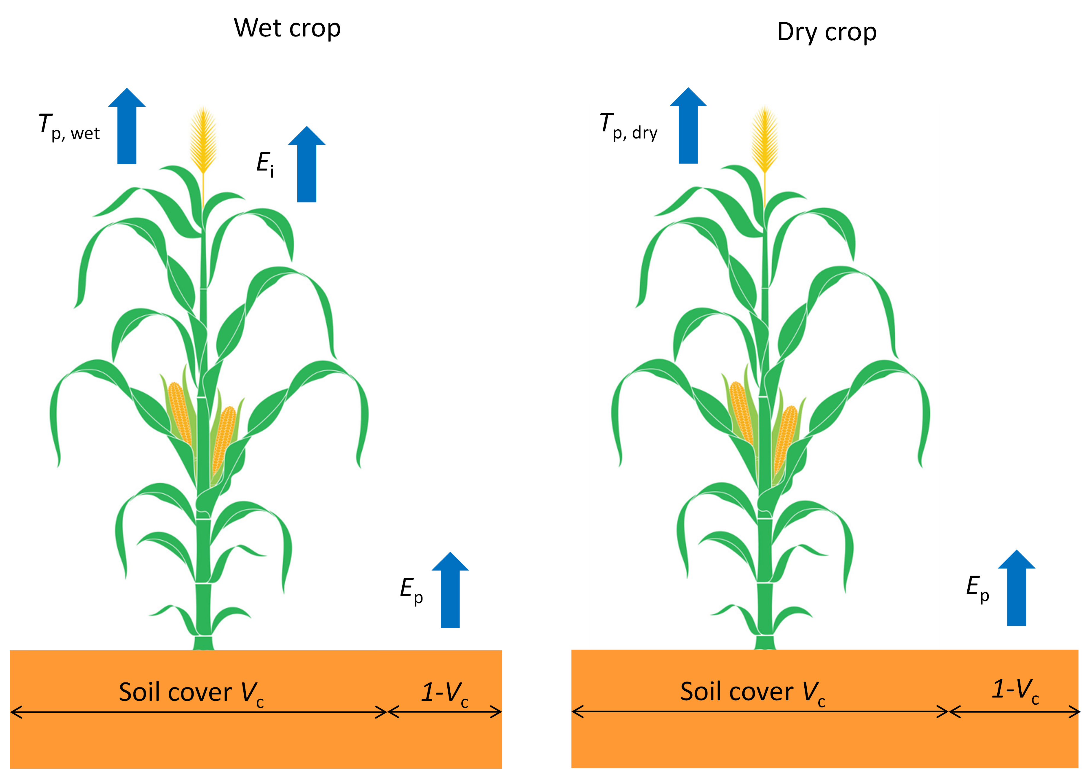
\[ T_\text{p,dry}=V_\text{c}ET_\text{p0} \tag{3.21}\] \[ ET_\text{wet}=V_\text{c}ET_\text{w0} \tag{3.22}\]
\[ E_\text{p}=\left(1-V_\text{c}\right)E_\text{p0} \tag{3.23}\]
where \(V_\text{c}\) represents the vegetation cover (-).
3.4.3 Transpiration and evaporation rate of a wet canopy
During the time a vegetation is wet, both transpiration through the stomata and evaporation of intercepted water on the leaves will occur. The more solar energy is used for transpiration through the stomata, the less solar energy is left for evaporation of intercepted water on the leaves. SWAP weights both fluxes as follows:
\[ T_\text{p,wet} = \frac{T_\text{p,dry}}{T_\text{p,dry}+ET_\text{wet}} T_\text{p,dry} \tag{3.24}\]
\[ E_\text{i} = \frac{ET_\text{wet}}{T_\text{p,dry}+ET_\text{wet}} ET_\text{wet} \tag{3.25}\]
where \(T_\text{p,wet}\) is the potential transpiration rate of hte wet canopy an d \(E_\text{i}\) the evaporation rate of a wet canopy.
Therefore the fraction of a day that the canopy is wet can be calculated as:
\[ W_\text{frac} = \frac{P_\text{i}}{E_\text{i}} \quad \text{with} \quad W_\text{frac} \le 1.0 \tag{3.26}\]
where \(P_\text{i}\) is the rainfall interception (mm d-1) and \(E_\text{i}\) is the evaporation flux of a wet canopy (mm d-1).
In case of Rutter, \(W_\text{frac}\) = 1.0 as long there is water stored in the canopy reservoir and \(W_\text{frac}\) = 0.0 if the canopy reservoir is empty. When \(E_\text{i}\) exceeds the incoming rainfall, SWAP assumes a semi-wet canopy:
\[ W_\text{frac} = \frac{V_\text{c}P_\text{g}}{E_\text{i}} \tag{3.27}\]
3.4.4 Potential transpiration
The transpiration and evaporation fluxes determined until here with either direct application of Penman-Monteith or based on reference evapotranspiration with crop and soil factors, are depicted in Figure 3.5.
Finally, the most important flux for soil hydrology and crop growth can be determined: the potential transpiration during the entire day. Taking into account the day fraction during which the crop is wet, this flux can be calculated as follows:
\[ T_\text{p} = W_\text{frac} T_\text{p,wet} + \left(1 -W_\text{frac} \right)T_\text{p,dry} \tag{3.28}\]
3.5 Actual plant transpiration
3.5.1 General approach
The potential transpiration and evaporation fluxes (\(T_\text{p}\) and \(E_\text{p}\)) as described in Section 3.4 are based on atmospheric conditions and vegetation properties, assuming favourable soil moisture conditions. In this paragraph, we describe the reduction of root water uptake and thus transpiration due to oxygen stress and drought stress. In Section 3.6, the reduction of soil evaporation due to drying of the topsoil is described. Section 8.5 considers the effect of high salt concentrations on root water uptake and Section 10.2 the effect of frozen soils. Ultimately the calculations yield the actual transpiration and evaporation fluxes (\(T_\text{a}\) and \(E_\text{a}\)) as depicted in Figure 3.4.
The maximum possible root water extraction rate, integrated over the rooting depth, should equal \(T_\text{p}\) (cm d-1). Taking into account the root length density distribution (Bouten 1992), the potential root water extraction rate at a certain depth, \(S_\text{p}(z)\) (d-1), can be calculated by:
\[ S_\text{p}(z) = \frac{l_\text{root}(z)}{\int_{-D_\text{root}}^0 l_\text{root}(z) \partial z} T_\text{p} \tag{3.29}\]
where \(D_\text{root}\) is the root layer thickness (cm).
These potential fluxes to the roots are reduced due to suboptimal soil conditions: too wet, too dry, too saline, or too cold. SWAP determines stress factors for these factors at each soil compartment. In case of combined water and salt stress, Skaggs et al. (2006) argue that the stress factors for water and salt stress can be multiplied. In SWAP, we follow this multiplication approach for all stresses and calculate the actual root water flux, \(S_\text{a}(z)\) (d-1), as:
\[ S_\text{a}(z) = \alpha_\text{rw} \alpha_\text{rd} \alpha_\text{rs} \alpha_\text{rf} S_\text{p}(z) \tag{3.30}\]
where \(\alpha_\text{rd}\) (-), \(\alpha_\text{rw}\) (-), \(\alpha_\text{rs}\) (-), and \(\alpha_\text{rf}\) (-) are the reduction factors for conditions that are too wet, too dry, too saline, or too cold, respectively.
Integration of \(S_\text{a}(z)\) over the root layer yields the actual transpiration rate \(T_\text{a}\) (cm d-1):
\[ T_\text{a} = \int_{-D_\text{root}}^0 S_\text{a}(z) \partial z \tag{3.31}\]
In many applications, the proportion of occurring stress factors is relevant information. Therefore, SWAP will split the total transpiration reduction into individual contributions of the occurring stress factors by multiplying (\(S_p(z) - S_a(z)\)) with the proportion of the logarithmic value of each of the reduction factors \(\frac{\log(\alpha_\text{j})}{\sum_\text{i=1} \log(\alpha_\text{i})}\).
3.5.2 Feddes function for root water uptake
Stresses due to dry or wet conditions and/or high salinity concentrations may reduce \(S_\text{p}(z)\). The water stress in SWAP is described by the function proposed by Feddes, Kowalik, and Zaradny (1978), which is depicted in Figure 3.6. In the range \(h_\text{3}\) < \(h\) < \(h_\text{2}\), root water uptake is optimal. Below \(h_\text{3}\), root water uptake linearly declines due to drought until zero at \(h_\text{4}\) (wilting point). The critical pressure head \(h_\text{3}\) increases for higher potential transpiration rates \(T_\text{p}\) (critical pressure head values according to Taylor and Ashcroft (1972) are provided in Appendix G). Above \(h_\text{2}\), root water uptake linearly declines due to insufficient aeration until zero at \(h_\text{1}\), i.e., representing threshold values for minimum and maximum oxygen deficiency.
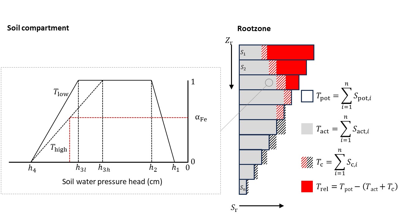
The total water demand (\(T_{\text {pot}}\), cm d-1) is divided over all soil layers proportional to a given root distribution. For each soil compartment, the actual water uptake is calculated as described above. The sum of uptake from all the compartments (\(T_{\text {act}}\), cm d-1) is then compared to the total demand to determine the amount of reduction (if any). Compensation, i.e., more uptake from a wet layer if one or more other layers present a reduced uptake, may be included according to Jarvis (1989, 2011), which is visualized in Figure 3.6 (right). If \(\alpha_{\text {crit}}\) <= \(T_{\text {act}}\)/\(T_{\text {pot}}\) < 1, where \(\alpha_{\text {crit}}\) is a user-defined value in the range [0…1] (e.g., \(\alpha_{\text {crit}}\) = 0.7), complete compensation is simulated and for each soil compartment the actual root water uptake is multiplied by the factor \(T_{\text {pot}}\)/\(T_{\text {act}}\), such that \(T_{\text {act,c}}\) = \(T_{\text {pot}}\) (subscript c refers to the result after applying compensation). If \(T_{\text {act}}\)/\(T_{\text {pot}}\) < \(\alpha_{\text {crit}}\), partial compensation is simulated: for each compartment, the uptake is multiplied by \(1/\alpha_{\text {crit}}\), which results in \(T_{\text {act,c}}\) = \(T_{\text {act}}\)/\(\alpha_{\text {crit}}\) < \(T_{\text {pot}}\).
Constant critical pressure heads for oxygen stress seem not realistic, as oxygen stress depends on various abiotic and biotic factors. Therefore, as an alternative, the process-based method of Bartholomeus et al. (2008) has been implemented (Section 3.5.3). At the dry side, the input values for \(h_\text{3l}\) and \(h_\text{3h}\) depend on plant type, soil texture, root density, and atmospheric demand, input values which are not commonly available. Also, the linear decline of the reduction factor in the range \(h_\text{4}\) < \(h\) < \(h_\text{3}\) may deviate from reality. Therefore, also a detailed, microscopic root water uptake module for drought has been added to SWAP (Section 3.5.4).
3.5.3 Detailed oxygen stress
When the availability of oxygen or water is insufficient to meet the metabolic demands of plants for these resources, the plant suffers from oxygen and drought stress, respectively. The first physiological process inhibited at oxygen stress (resulting from high soil moisture contents) is plant root respiration, i.e., oxygen consumption in the roots, a process that increases with rising temperatures. High soil moisture contents hamper oxygen transport from the atmosphere, through the soil - where part of the oxygen is additionally consumed by soil microorganisms - and to the root cells. Reduced respiration negatively affects the energy supply to plant metabolism (Bartholomeus et al. 2011).
Root respiration is determined by interacting respiratory (i.e., oxygen consuming) and diffusive (i.e., oxygen providing) processes in and to the soil. Plant roots respire at a potential rate under optimal soil aeration and thus non-limiting oxygen availability. This potential root respiration is in equilibrium with the oxygen demand of plant roots, which is determined by plant characteristics and soil temperature (as simulated with SWAP). Upon increasingly wetter conditions, however, the gas-filled porosity of the soil decreases and oxygen availability becomes insufficient for potential root respiration. Daily respiration reduction (i.e., potential minus actual respiration) is calculated with a model for oxygen transport and consumption, which uses generally applied physiological and physical relationships to calculate both the oxygen demand of, and the oxygen supply to plant roots. For details and equations of the implemented method we refer to Bartholomeus et al. (2008).
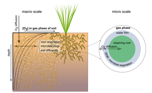
Simulation of the actual root respiration for a crop requires actual data on soil type, daily soil temperature, and daily gas-filled porosity in each soil layer. The latter two variables are simulated within SWAP. Simulation of soil temperature should thus be switched on. The model of Bartholomeus et al. (2008) is applied to all soil layers of SWAP, to account for layer-specific soil physical properties, moisture contents, and temperatures. The difference between potential and actual root respiration is calculated for each soil layer separately. Subsequently, the reduction coefficient \(\alpha_\text{rw}\) due to oxygen stress is calculated for each soil layer, based on the assumption that root water uptake is proportional to growth respiration.
The latter assumption is supported by several arguments (Bartholomeus et al. 2008). If stomata are fully opened, root water uptake is optimal (\(\alpha_\text{rw}\) = 1) and dominated by hydraulic forces. At fully open stomata, potential photosynthesis is achieved, and oxygen is needed for both maintenance and growth respiration. Potential root water uptake is thus only possible as long as there is no oxygen stress. Oxygen stress induces stomatal closure (e.q., Glínski and Stępniewksi 1985; Kramer 1951). At complete stomatal closure, the actual transpiration and photosynthesis approach zero (\(\alpha_\text{rw}\) = 0). In that case, oxygen is solely used for maintenance respiration. Between the limits \(\alpha_\text{rw}\) = 1 and \(\alpha_\text{rw}\) = 0, it is assumed that the reduction of root water uptake is directly proportional to the reduction in root respiration. Kamaluddin and Zwiazek (2001) demonstrated, by inhibition of the metabolism of the roots, that a positive correlation between root respiration and water uptake exists. This implies a gradual decrease of root water uptake with increased oxygen stress (Bartholomeus et al. 2008).
3.5.4 Detailed drought stress
Besides the macroscopic root water uptake model by Feddes, several process-based models describing root water uptake have been published. Two of these have been implemented in SWAP. De Willigen and Van Noordwijk (1987) described the process of uptake by roots; not only of water but also of oxygen (see above) and nutrients. Around each root a cylindrical soil column can be assumed with root radius \(R_0\) (cm); the radius of this soil cylinder is inversely proportional to the root length density according to (Figure 3.8; left)
\[ R_1 = \left (\pi {L_{\text {rv}}} \right )^{-0.5} \tag{3.32}\]
where \(R_1\) is the radius of the soil cylinder (cm) and \(L_{\text {rv}}\) is the root length density (cm cm-3). Water will flow from the outside of the cylinder toward the root in the middle due to a gradient in pressure head (\(h\)) gradient (Figure 3.8; right).
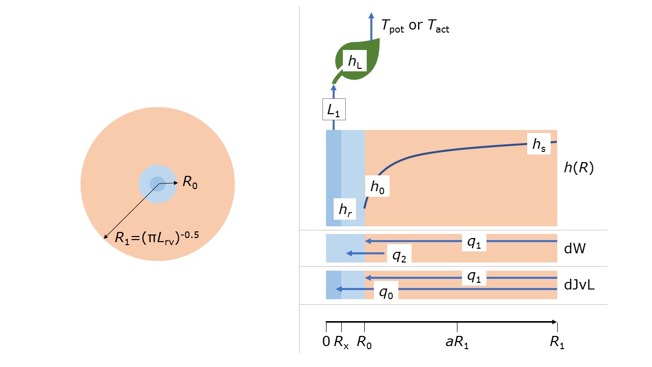
De Willigen and Van Noordwijk (1987) showed that the physical state in the soil column can be described very accurately with an analytical, steady-rate formulation. This formulation is not based on \(h\) but on the matric flux potential, \(M(h)\) (cm2 d-1), defined as the integral of \(K(h)\) (Raats 1970). Any profile described in terms of \(M\) can be transformed in \(h\) or \(\theta\). The analytical solution provides an expression for the water flux \(q\) (cm3 cm-2 d-1) towards the root wall and can be upscaled to an entire root system. For that purpose, De Willigen and Van Noordwijk (1991), Heinen (2001) and De Willigen et al. (2011, 2012) (further denoted as the dW concept) used two fluxes: a water flux in the soil column towards the root wall (\(q_1\)) and a water flux across the root wall (\(q_2\)) (Figure 3.8). For the dW concept, the equations involved are given by
\[ q_{1,j} = \Delta z_j \rho_{\text {dW},j}(M_{\text s,j} - M_{\text 0,j}) \tag{3.33}\]
where \(q_1\) is the flux from the bulk soil (s) toward the root-soil interface (0) (cm d-1), \(\Delta z\) is the thickness of the soil compartment (cm), \(M\) is the matric flux potential (cm2 d-1), \(j\) is the soil compartment sequential number, and \(\rho_{\text {dW}}\) is a geometry factor (cm-2) given by
\[ \rho_{\text {dW}} = \frac{(r^2 - 1)} {0.5R_1^2 \left( 0.25(1 - 3r^2)+r^4\ln \left( \frac{r} {r^2 - 1} \right) \right)} \tag{3.34}\]
with
\[ r = \frac{R_1} {R_0} \tag{3.35}\]
The water flux across the root wall \(q_2\) (cm d-1) is given by
\[ q_{2,j} = \Delta z_j L_{\text {rv},j}K_{\text r}(h_{0,j} - h_{r}) \tag{3.36}\]
where \(K_r\) is the hydraulic conductivity of the root wall (cm d-1), and \(h_{\text r}\) is root water potential (cm). The \(h_{\text r}\) is related to the leaf water potential \(h_{\text L}\) via a relationship taken from Zhuang et al. (2001)
\[ h_{\text L} = h_{\text r} - \frac{T_{\text {pot}}} {a_0 + a_1 T_{\text {pot}}} \tag{3.37}\]
with \(a_0\) = 3.1844 10-5 d-1 en \(a_1\) = 1.7768 10-4 cm-1 (De Willigen et al. 2011). The transpiration reduction function is given by (Campbell 1991)
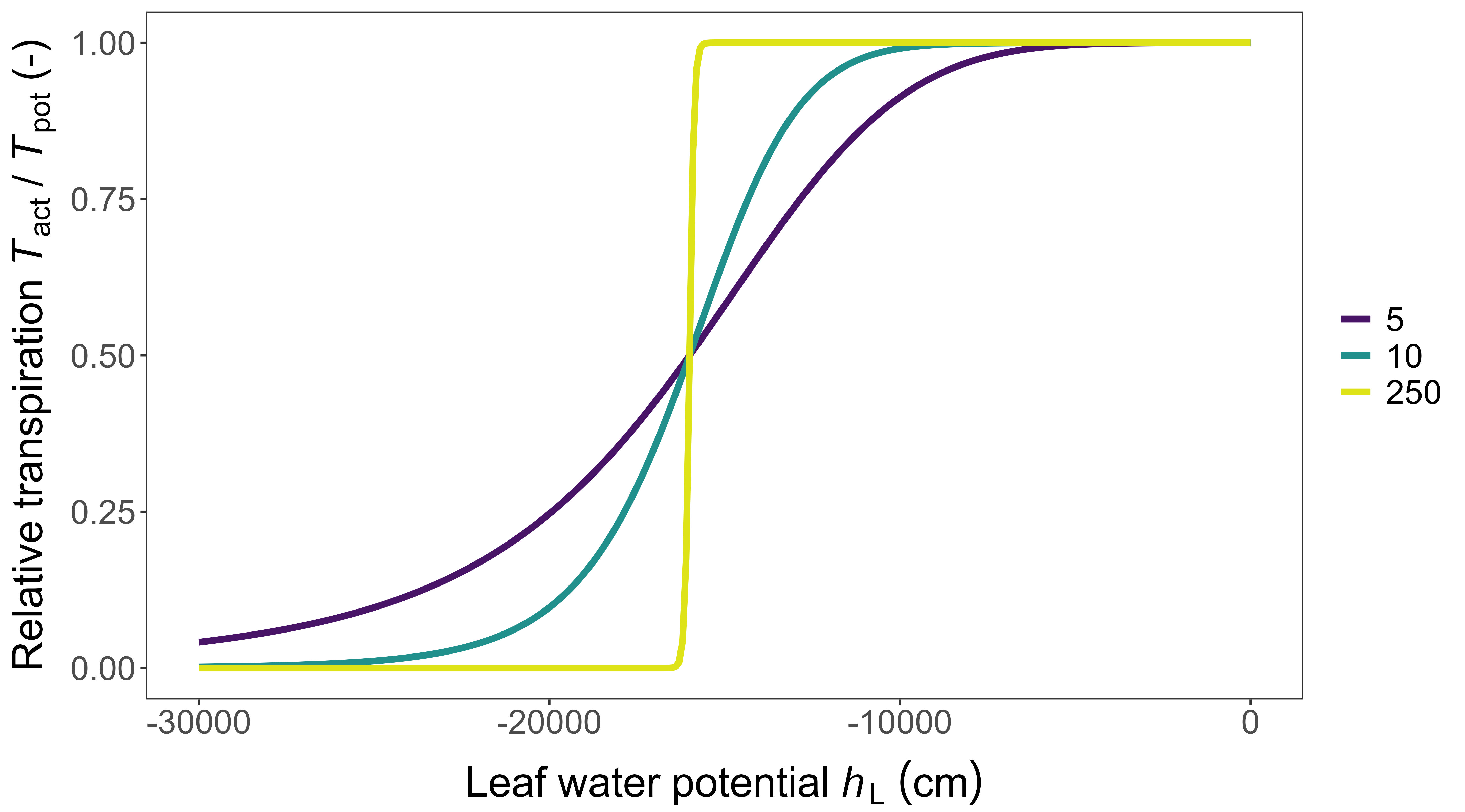
\[ T_{\text{act}} = T_{\text{pot}} \left (1 + \left (\frac{h_{\text L}} {h_{\text L,1/2}} \right )^{\text p} \right )^{-1} \tag{3.38}\]
where \(h_{\text L,1/2}\) is \(h_{\text L}\) where \(T_{\text {act}}\) = 0.5\(T_{\text {pot}}\), and \(p\) is a dimensionless curve shape parameter, usually in the range 5 to 10; a step function can be approximated by taking a large value for \(p\) (e.g., \(p\) = 250) (Figure 3.9). The sum for all computational layers of all \(q_1\) and that of all \(q_2\) must be equal to each other and equal to the (actual) water uptake \(T_{\text {act}}\)
De Jong van Lier et al. (2013) used the same steady-rate solution (further denoted as the dJvL concept). They defined an alternative expression for the water flux from the soil column directly into the root (\(q_0\)) which also includes \(q_1\). For the dJvL concept, the main equation is given by
\[ h_{0,j} + \phi_{\text {dJvL},j}M_{0,j} = h_{\text L}+\phi_{\text {dJvL},j}M_{\text {s},j}+ \frac{T_{\text {act}}} {L_1} \tag{3.39}\]
where \(L_1\) is the conductance in the pathway root-stem-leave (d-1) and \(\phi_{\text{dJvL}}\) is a geometry factor (d cm-1) given by
\[ \phi_{\text{dJvL}} = \frac {R_1^2\ln \left ( \frac {R_0} {R_x} \right )} {2K_{\text r}} \rho_{\text{dJvL}} \tag{3.40}\]
where \(R_{\text x}\) is the radius of the xylem vessel (cm) and \(\rho_{\text {dJvL}}\) is a geometry factor (cm-2) given by
\[ \rho_{\text{dJvL}} = \frac {4} {R_0^2-a^2R_1^2+2 \left ( R_0^2 + R_1^2\right ) \ln \left ( \frac {aR_1} {R_0} \right )} \tag{3.41}\]
where \(a\) is a dimensionless fraction indicating where in the soil cylinder the pressure head equals the value \(h_{\text s}\). According to De Jong van Lier et al. (2006; 2008, 2013) \(a\) = 0.53 is a good approach in monomodal Van Genuchten-type soils.
The water flux inside the soil cylinder is given by
\[ q_{1,j} = \Delta z_j\rho_{\text{dJvL}} \left ( M_{\text s,j} - M_{o,j} \right ) \tag{3.42}\]
Both the concepts of dW and dJvL result in a set of \(N\) non-linear equations with \(N\) unknowns, with the requirement that the sum of water uptake from all soil compartments is equal to \(T_{\text {act}}\), the latter being a function of the additional unknown \(h_{\text L}\). The \(N\) unknowns are \(h_0\) (note: \(M_0\) is a function of \(h_0\)) and the non-linearity is a consequence of the non-linear functions \(M(h)\) and \(T_{\text {act}}(h_{\text L})\). This equation system is solved via a double, nested iteration procedure as described in Appendix H.
For both the concepts of dW and dJvL implicit compensation occurs. By simultaneously solving the system for all computational layers in the root zone, a thermodynamically most favourable distribution of water uptake is simulated: more water uptake will implicitly be simulated from zones where hydraulic conditions are more favourable, and no subsequent computational step is needed to deal with this compensation (De Willigen et al. 2011).
3.6 Actual soil evaporation
At a wet soil, soil evaporation equals its potential rate \(E_\text{p}\). This is also the case at ponded conditions, during which SWAP will increase \(E_\text{p}\) to the evaporation rate of intercepted water with or without a ponding factor (Table 3.2). When the soil becomes drier, the soil hydraulic conductivity decreases, which may reduce \(E_\text{p}\) to evaporation rate, \(E_\text{a}\) (cm d-1). In SWAP, the maximum evaporation rate that the top soil can sustain, \(E_{\text{max}}\) (cm d-1), is calculated according to Darcy’s law:
\[ E_{\text{max}} = K_\text{½} \left( \frac{h_{\text{atm}} - h_1 - z_\text{1}}{z_\text{1}} \right) \tag{3.43}\]
where \(K_\text{½}\) is the average hydraulic conductivity (cm d-1) between the soil surface and the first node, \(h_\text{atm}\) is the soil water pressure head (cm) in equilibrium with the air relative humidity, \(h_\text{1}\) is the soil water pressure head (cm) of the first node, and \(z_\text{1}\) is the soil depth (cm) at the first node. Equation 3.43 excludes water flow due to thermal differences in the top soil and due to vapour flow, as on daily basis the concerned flow amounts are probably negligible compared to isothermal, liquid water flow (Koorevaar, Menelik, and Dirksen 1983; Ten Berge 1986; Jury, Gardner, and Gardner 1991). Note that the value of \(E_\text{max}\) in Equation 3.43 depends on the thickness of the top soil compartments. Increase of compartment thickness, generally results in smaller values for \(E_\text{max}\) due to smaller hydraulic head gradients. For accurate simulations at extreme hydrological conditions, the thickness of the top compartments should not be more than 1 cm (Van Dam and Feddes 2000).
There is one serious limitation of the \(E_\text{max}\) procedure as described above. \(E_\text{max}\) is governed by the soil hydraulic functions \(\theta (h)\) and \(K(\theta)\). It is still not clear to which extent the soil hydraulic functions, that usually represent a top layer of a few decimeters, are valid for the top few centimeters of a soil, which are subject to splashing rain, dry crust formation, root extension and various cultivation practices, including mulch additions. Therefore also empirical evaporation functions may be used, which require calibration of their parameters for the local climate, soil, cultivation and drainage situation. SWAP has the option to choose the empirical evaporation functions of Black, Gardner, and Thurtell (1969) or Boesten and Stroosnijder (1986).
Reduction of soil evaporation according to Black
Black, Gardner, and Thurtell (1969) calculated the cumulative actual evapotranspiration during a drying cycle, \(\sum E_a\) (cm) as:
\[ \sum E_\text{a} = \beta_\text{1} t_{\text{dry}}^{½} \tag{3.44}\]
where \(\beta_\text{1}\) is a soil-specific parameter (cm d-½), characterizing the evaporation process and \(t_{\text{dry}}\) is the time (d) after a significant amount of rainfall, \(P_{\text{min}}\). SWAP resets \(t_{\text{dry}}\) to zero if the net precipitation \(P_{\text{net}}\) exceeds \(P_{\text{min}}\).
Reduction of soil evaporation according to Boesten and Stroosnijder
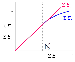
The Black-parameter \(\beta_1\) will be affected by the potential evaporation rates in the drying period. Therefore Boesten and Stroosnijder (1986) proposed to replace time by the sum of potential evaporation, \(\sum E_p\) (cm), as time variable (Figure 3.10):
\[ \sum E_\text{a} = \begin{cases} \sum E_\text{p} & \text{for} \space \sum E_\text{p} \le \beta_\text{2}^\text{2} \\ \beta_\text{2} \left(\sum E_\text{p}\right)^{½} & \text{for} \space \sum E_\text{p} > \beta_\text{2}^\text{2}\\ \end{cases} \tag{3.45}\]
where \(\beta_\text{2}\) is a soil parameter (cm½), which should be determined experimentally. The parameter \(\beta_\text{2}\) determines the length of the potential evaporation period, as well as the slope of the \(\sum E_\text{a}\) versus \((\sum E_\text{p})^½\) relationship in the soil limiting stage.
Boesten and Stroosnijder suggest the following procedure with respect to updates of \(\sum E_\text{p}\). On days with no excess in rainfall (\(P_\text{net} < E_\text{p}\)), \(\sum E_\text{p}\) follows from Equation 3.45:
\[ \left(\sum E_\text{p}\right)^j = \left(\sum E_\text{p}\right)^\text{j-1} + \left(E_\text{p} - P_\text{net}\right)^\text{j} \tag{3.46}\]
where \(j\) is the day number. \((\sum E_\text{a})^\text{j}\) is calculated from \((\sum E_\text{p})^\text{j}\) with Equation 3.45, and \(E_\text{a}^\text{j}\) is calculated with:
\[ E_\text{a}^\text{j} = P_\text{net}^\text{j} + \left(\sum E_\text{a}\right)^\text{j} - \left(\sum E_\text{a}\right)^\text{j-1} \tag{3.47}\]
On days of excess rainfall (\(P_{\text{net}} > E_\text{p}\)):
\[ E_\text{a}^\text{j} = E_\text{p}^\text{j} \tag{3.48}\]
and the excess rainfall is subtracted from \(\sum E_\text{a}\):
\[ \left(\sum E_\text{a}\right)^\text{j} = \left(\sum E_\text{a}\right)^\text{j-1} - \left(P_\text{net} - E_\text{p}\right)^\text{j} \tag{3.49}\]
Next \(\left(\sum E_\text{p}\right)^\text{j}\) is calculated from \(\left(\sum E_\text{a}\right)^\text{j}\) with Equation 3.45. If the daily rainfall excess is larger than \(\left(\sum E_\text{p}\right)^\text{j-1}\), then both \(\left(\sum E_\text{a}\right)^\text{j}\) and \(\left(\sum E_\text{p}\right)^\text{j}\) are set to zero.
SWAP will determine \(E_\text{a}\) by taking the minimum value of \(E_\text{p}\), \(E_\text{max}\), and, if selected by the user, one of the empirical functions.
3.7 User Instructions
3.7.1 General Information
Tip 3.1 lists the general input data required for calculating evapotranspiration. A main choice is whether pre-calculated \(ET_\text{ref}\) values are used (swetr = 1) or whether evapotranspiration is calculated from basic meteorological data, i.e. on solar radiation, air temperature, air humidity and wind speed. These basic weather data can be specified as daily values or at shorter, constant time intervals (swmetdetail = 1).
When daily meteorological data are used, SWAP can distribute the evapotranspiration flux uniformly over the day or according to a sine wave over the photoperiod (SWMETSINE = 1) using constant time intervals (NMETSINE). As listed in Tip 3.1, the rainfall input may range from daily amounts to short time rainfall amounts.
As described in Section 3.4, the partitioning of potential transpiration and evaporation fluxes can be based on crop and soil factors, or on direct application of the Penman-Monteith equation. With swdivide the user selects the preferred method. For many applications daily input of solar radiation, air temperature, air humidity and (daytime) wind speed is preferred. In that case SWAP may apply the Penman-Monteith method to determine \(ET_\text{p}\). If some of these data are missing or unreliable, alternative methods to determine \(ET_\text{ref}\) in combination with crop factors are advised.
Input of daily rainfall amounts will suffice for most applications. However, when surface runoff is expected, daily rainfall amounts may underestimate the amount of surface runoff. To calculate surface runoff, actual rainfall intensities should be used.
3.7.2 Weather data
In case of daily weather records, the data should be specified as listed in Tip 3.2. Missing data are given the number -99.9. When SWAP uses Penman Monteith (swetr = 0), data on solar radiation, air temperature (min and max), air humidity and (daytime) wind speed are required. When SWAP should simulate detailed crop growth (Chapter 7), data on solar radiation and air temperature (min and max) are required. For rainfall, either daily amounts (swrain = 0) or daily amounts plus duration (swrain = 2) should be specified.
Alternatively weather records can be specified with short, constant time intervals (> 15 minutes) according to the format listed in Tip 3.3. Radiation and rainfall denote total amounts during the time interval. Air temperature, humidity and wind speed denote average values during the time interval.
A third combination is daily evapotranspiration data and detailed rainfall data. In this case evapotranspiration data are input according to Tip 3.2, while the rainfall data are input according to Tip 3.4. The rainfall data follow the format of a tipping bucket measurement device: the rainfall amount corresponds to the total amount in the previous period.
3.7.3 Soil data
Tip 3.5 lists the soil data which are required to determine the actual evaporation at the soil surface. The soil factor (cfbs) can be used to transform reference crop evapotranspiration into potential soil evaporation (see Section 3.3.2 and Table 3.2). Commonly a soil factor cfbs = 0.5 is used.
Three options are offered to reduce soil evaporation according to the maximum water flux which can be delivered by the soil. Applying straight soil physical theory, the maximum soil water flux according to Darcy would suffice. However, as discussed in Section 3.6, this method in general overestimates actual soil evaporation. Therefore, we recommend to use in addition to the Darcy flux, reduction with either the Black or Boesten and Stroosnijder method (swredu = 1 or 2).
Default soil evaporation coefficient for Black equals 0.35 cm d-0.5, and for Boesten and Stroosnijder 0.54 cm0.5.
3.7.4 Plant data
The required plant input data to calculate evapotranspiration and rainfall interception will be listed at the end of Chapter 7. The theory in this chapter and the description in the input file should be sufficient to provide the proper input values for most variables. In this section we provide more information on the input for the detailed oxygen module (Section 3.5.3) and the detailed drought stress module (Section 3.5.4).
Detailed oxygen stress The oxygen module calculates the root uptake reduction factor \(\alpha_\text{rw}\) as function of plant characteristics and plant physiological processes, rooting depth, gas filled porosity, soil temperature, soil physical properties and soil microbial activity. Most input parameters required for the oxygen module (Table 3.3) are already standard input to SWAP simulations. When SWAP is used with the static crop module, crop development is input and plant physiological processes are not simulated. Consequently, for the simulation of oxygen stress some additional crop parameters are required of i) characteristics of the plant roots to simulate the root oxygen demand and ii) soil characteristics to simulate the oxygen consumption by soil microbial activity (Table 3.3, column ‘Static’). Using dynamic crop development decreases the number of extra input parameters from nine to four (Table 3.3, column ‘Dynamic’).
Using dynamic crop development (WOFOST) allows to describe the plant physiological processes, that determine the oxygen demand of plant roots, in more detail than with the static crop module. The following variables are relevant: - rooting depth - root biomass - ratio total root respiration : maintenance respiration
WOFOST simulates rooting depth and root biomass dynamically (daily). Root biomass is used to simulate the root maintenance respiration. The oxygen module calculates total root respiration from the maintenance respiration by multiplication with a factor \(\eta\): the ratio of total respiration and maintenance respiration (Bartholomeus et al. 2008). The factor \(\eta\) is derived on a daily basis from root growth respiration and maintenance respiration as simulated with WOFOST. For simulations with the simple crop module, \(\eta\) is an input variable.
It should be noted that WOFOST uses air temperature to simulate the temperature dependence of the plants’ maintenance respiration. This also holds for the simulation of root respiration. Within the oxygen module however, maintenance respiration is simulated with soil temperature as input.
Table 3.4 provides oxygen stress parameter values for a static grass crop; Table 3.5 provides parameter values for dynamic crop growth simulation (WOFOST, see Chapter 7) for the crops grass, potato and maize.
| Name of parameter | Description of parameter | Unit | Static crop | Dynamic crop |
|---|---|---|---|---|
| Q10_ROOT | Relative increase in root respiration at temperature increase of 10 °C | - | x | |
| Q10_MICROBIAL | Relative increase in microbial respiration at temperature increase of 10 °C | - | x | x |
| SPECIFIC_RESP_HUMUS | Specific respiration rate of humus at 25 °C | kg O2 kg-1 C d-1 | x | x |
| C_MROOT | Maintenance coefficient of root | kg O2 k-1 d-1 | x | |
| RTD | Root tissue density | g cm-3 | x | x |
| ROOTRADIUS | Root radius | cm | x | x |
| F_SENES | Reduction factor for senescence, used for maintenance respiration | - | x | |
| WROOTTB | Dry weight of roots [kg m-3] as a function of DVS | kg m-3 | x | |
| MRFTB | Ratio root total respiration / maintenance respiration as function of development stage | - | x |
| Name of parameter | Source | Value |
|---|---|---|
| Q10_ROOT | Amthor (2000) | 2.0 |
| Q10_MICROBIAL | Fierer et al. (2006) | 2.8 |
| SPECIFIC_RESP_HUMUS | Fierer et al. (2006) | 1e-3 |
| C_MROOT | Kroes et al. (2009) | 0.016 |
| RTD | De Willigen and Noordwijk (1987) | 0.1475 |
| ROOTRADIUS | De Willigen and Noordwijk (1987); Wopereis (1994); Deru, Eekeren, and Boer (2010) | 0.0075 |
| F_SENES | 1 | |
| MRFTB | Penning de Vries, Witlage, and Kremer (1979) | 5 |
| Name of parameter | Source | Crop | Value |
|---|---|---|---|
| Q10_MICROBIAL | Fierer et al. (2006) | 2.8 | |
| SPECIFIC_RESP_HUMUS | Fierer et al. (2006) | 1e-6 | |
| RTD | De Willigen and Noordwijk (1987) | grass | 0.1475 |
| potato | 0.0694 | ||
| maize | 0.0934 | ||
| ROOTRADIUS | De Willigen and Noordwijk (1987); Wopereis (1994); Deru, Eekeren, and Boer (2010) | grass | 0.0075 |
| Ehlert, Pasterkamp, and Brouwer (2004); De Willigen and Noordwijk (1987); Iwama (1998); Rawsthorne and Brodie (1986); Vos and Groenwold (1986) | potato | 0.014 | |
| De Willigen and Noordwijk (1987); Qin, Stamp, and Richner (2006) | maize | 0.015 |
Detailed drought stress Since governing input parameters for detailed drought stress (as well as for simple drought stress) are crop dependent, this information should be supplied via the crop input files which are described in Section 7.7.
Ranges of parameter values for the different parameters in both process-based root water uptake models (dW, dJvL) are presented in Table 3.6.
| Parameter | dW | dJvL | Description |
|---|---|---|---|
| \(R_0\) | + | + | Root radius (cm). Referring to the literature De Jong van Lier et al. (2013) stated that \(R_0\) lies often in the range 0.005 to 0.05 cm; they used \(R_0\) = 0.05 cm. De Willigen et al.(2012) used \(R_0\) = 0.075 cm, and . (De Willigen, Heinen, and Noordwijk 2017) used \(R_0\) = 0.01 cm. De Willigen & van Noordwijk (1987) summarized \(R_0\) from a literature review: grains: 0.009-0.0165 cm, maize 0.0095-0.0105 cm, grass: 0.005- 0.0145 cm, potato: 0.014 cm. Spek (2008) published measured \(R_0\) for main roots in the range 0.034 – 0.054 cm and for secondary roots in the range 0.0084 – 0.0124 cm. De Willigen et al. (2005) stated that \(R_0\) is of little influence on the radial resistance for water flow inside the root as well as for the required pressure head gradient in the soil cylinder surrounding the root. |
| \(R_1\) | + | + | Radius of soil cylinder surrounding the root (cm). Calculated according to Equation 3.33. Based on literature data De Willigen & van Noordwijk (1987) listed \(L_{rv}\) data for the 0-30 cm layer for some crops: bean: 0.5-2 cm cm-3, potato: 1-2 cm cm-3, sugar beet : 1-2 cm cm-3, maize: 3 cm cm-3, grains: 4-5 cm cm-3, grass: 3-20 cm cm-3. |
| \(R_x\) | - | + | Radius of xylem vessel (cm). According to De Jong van Lier et al. (2013) the range \(R_x\)/\(R_0\) often is in the range 0.1 to 0.9, based on root morphological observations. They used \(R_x\) = 0.02 cm and \(R_0\) = 0.05 cm |
| \(a\) | - | + | Based on numerical analyses De Jong van Lier et al. (2006; 2008, 2013) concluded that \(a\) can be considered constant with \(a\) = 0.53. |
| \(K_r\) | + | + | Hydraulic conductivity of the root wall (cm d-1). De Willigen et al. (2012) used \(K_r\) = 8.143 10-5 cm d-1; De Willigen et al. (2017) used \(K_r\) = 3.6 10-6 cm d-1. De Jong van Lier et al. (2013) gave a range between 4 10-8 to 3 10-5 cm d-1, and they used 3.5 10-6 cm d-1. De Willigen & van Noordwijk (1987) gave a range between 0.26 10-6 to 23.3 10-6 cm d-1, and specifically for maize and grains a range between 0.26 10-6 to 5.9 10-6 cm d-1 |
| \(L_1\) | - | + | Conductance of the pathway root-stem-leave (d-1). Based on data from Zhuang et al (2001) De Jong van Lier et al. (2013) gave \(L_1\) = 0.7 10-4 d-1 for \(T_{pot}\) = 2 mm d-1 and \(L_1\) = 2.1 10-4 d-1 for \(T_{pot}\) = 10 mm d-1. They used an average value of \(L_1\) = 1 10-4 d-1. NB: \(L_1\) = \(a_0\) + \(a_1 T_{pot}\), with \(a_0\) and \(a_1\) as described below. The value \(L_1\) = 1 10-4 d-1 corresponds to \(T_{pot}\) of about 4 mm d-1 |
| \(a_0\) | + | - | \(a_0\) = 3.1844 10-5 d-1 based on data of Zhuang et al. (2001) according to De Willigen et al. (2011, 2012). |
| \(a_1\) | + | - | \(a_1\) = 1.7768 10-4 cm-1 based on data of Zhuang et al. (2001) according to De Willigen et al. (2011, 2012). |
| \(h_w\) | - | + | Leaf water potential where reduction in root water uptake occurs according to the step-function of De Jong van Lier et al. (2013). They used \(h_w\) = -150000 cm or -20000 cm. See also \(h_{L,1/2}\) |
| \(h_{L,1/2}\) | + | + | Leaf water potential where the reduction in root water uptake equals 0.5 (cm). Based on Kremer et al. (2008) De Willigen et al. (2012) gave \(h_{L,1/2}\) = -16600 cm. De Jong van Lier et al. (2013) gave limiting leaf water potentials obtained from literature: maize: -17000 cm, purple bush bean: -7000 cm, sorghum: -20000 cm, tobacco: -13000 cm, rice: -8000 to -12000 cm. |
| \(p\) | + | + | Shape parameter (dimensionless). Based on Kremer et al. (2008) De Willigen et al. (2012) gave \(p\) = 7. Campbell (1991) indicated that \(p\) lies in the range 5 to 10. A step-function can be approximated by taking \(p\) large, e.g., \(p\) = 250. |