8 Solute transport
8.1 Introduction
Water is a great dissolver and many solutes enter the natural soil system at the Earth’s surface. The solute residence time in the unsaturated zone is important for soil and groundwater pollution management. For instance, organic compounds are mainly decomposed in the unsaturated zone, where the biological activity is concentrated. Most plants are able to extract water and nutrients from the soil only in the unsaturated zone. In irrigated areas, the long-term salinity in the root zone will depend on the amount of percolation from the unsaturated zone. Whereas in the unsaturated zone the transport of solutes is predominantly vertical, once being in the groundwater solutes may diverge in any direction, threatening surface waters, nature reserves, and drinking wells. Using an analytical model, Beltman, Boesten, and Zee (1995) show the importance of the transport processes in the unsaturated zone as compared to the transport processes in the saturated zone. It is clear that a thorough understanding is needed of the processes that govern the transport, adsorption, root uptake, and decomposition of the solutes in the unsaturated zone, in order to analyze and manage soil and water-related environmental problems.
SWAP is designed to simulate basic transport processes at the field scale level. Although for management purposes most farmers try to have more or less the same soil and drainage conditions per field, still the existing soil spatial heterogeneity within a field may cause a large variation of solute fluxes (Biggar and Nielsen 1976; Van de Pol, Wierenga, and Nielsen 1977; Van der Zee and Riemsdijk 1987). Most of this variation is caused by spatial variation of the soil hydraulic functions, preferential flow due to macropores in structured soils or unstable wetting fronts in unstructured soils. In many cases, it will not be possible to determine the variation (including the correlations) of all the physical parameters (Hopmans and Stricker 1989). SWAP confines to the physical processes in order to be flexible in parameter input and allow the simulation of all kinds of design and management scenarios. The spatial variability can be taken into account by inverse modeling or Monte Carlo simulation. Inverse modeling has been applied by Groen (1997). He measured for a period of time the solute concentrations in the soil profile and drainage water and determined ‘field effective’ transport parameters by inverse modeling. In case of Monte Carlo simulations, the model is run a large number of times, while the input parameters and boundary conditions are varied according to the variation at comparable fields (Boesten and Linden 1991).
SWAP focuses on the transport of salts, pesticides, and other solutes that can be described with relatively simple physical relations: convection, diffusion, dispersion, root uptake, Freundlich adsorption, and first-order decomposition. Transport related processes that are not considered in SWAP are:
- Volatilization and gas transport
- Transport of non-mixing or immiscible fluids (e.g., oil and water)
- Chemical equilibria of various solutes (e.g., between Na+, Ca2+, and Mg2+)
- Chemical and biological chain reactions (e.g., mineralization, nitrification)
In case of advanced pesticide transport, including volatilization and kinetic adsorption, SWAP can be used in combination with the model PESTLA (Van den Berg and Boesten 1998) and PEARL (Leistra et al. 2001; Tiktak et al. 2000). For nutrient transport (nitrogen and phosphorus), SWAP can be used in combination with the model ANIMO (Rijtema, Groenendijk, and Kroes 1997; Kroes and Roelsma 1997) or Soil-N (Groenendijk et al. 2016).
In this chapter, we first describe the solute transport processes that are considered in SWAP. Next, we discuss the boundary conditions applied. Also, we consider how SWAP deals with solute transport in water-repellent soils and in cracked clay soils. Salinization is a special case of solute transport. We describe the salinity stress options in SWAP. Finally, we provide an overview of solute transport input data.
8.2 Basic equations
8.2.1 Transport processes
The three main solute transport mechanisms in soil water are diffusion, convection, and dispersion. Diffusion is solute transport caused by the solute gradient. Thermal motion of the solute molecules within the soil solution causes a net transport of molecules from high to low concentrations. The solute flux \(J_{\text{dif}}\) (mg cm-2 d-1) is generally described by Fick’s first law:
\[ J_{\text{dif}} = -\theta D_{\text{dif}} \frac{\partial c}{\partial z} \tag{8.1}\]
with \(D_{\text{dif}}\) the diffusion coefficient (cm2 d-1) and \(c\) the solute concentration in soil water (mg cm-3). \(D_{\text{dif}}\) is very sensitive to the actual water content, as it strongly affects the solute transport path and the effective cross-sectional transport area. In SWAP we employ the relation proposed by Millington and Quirk (1961):
\[ D_{\text{dif}} = D_{\text{w}} \frac{\theta^{7/3}}{\phi_{\text{por}}^2} \tag{8.2}\]
with \(D_{\text{w}}\) the solute diffusion coefficient in free water (cm2 d-1) and \(\phi_{\text{por}}\) the soil porosity (cm3 cm-3).
The bulk transport of solutes occurs when solutes are carried along with the moving soil water. The mean flux of this transport is called the convective flux, \(J_{\text{con}}\) (mg cm-2 d-1), and can be calculated from the average soil water flux:
\[ J_{\text{con}} = qc \tag{8.3}\]
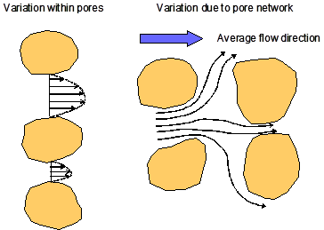
When describing water flow, we usually consider the Darcy flux \(q\) (cm d-1), which is averaged over a certain cross-section. In the case of solute transport, we have to account for the water velocity variation between pores of different sizes and geometry and also the water velocity variation inside a pore itself (Figure 8.1). The variety of water velocities causes some solutes to advance faster than the average solute front, and other solutes to advance slower. The overall effect will be that steep solute fronts tend to smoothen or disperse. Solutes seem to flow from high to low concentrations. If the time required for solutes to mix in the transverse direction is small, compared to the time required for solutes to move in the flow direction by mean convection, the dispersion flux \(J_{\text{dis}}\) (mg cm-2 d-1) is proportional to the solute gradient (Bear 1972):
\[ J_{\text{dis}} = -\theta D_{\text{dis}} \frac{\partial c}{\partial z} \tag{8.4}\]
with \(D_{\text{dis}}\) the dispersion coefficient (cm2 d-1). Under laminar flow conditions \(D_{\text{dis}}\) itself is proportional to the pore water velocity \(v = q/\theta\) (Bolt 1979):
\[ D_{\text{dis}} = L_{\text{dis}} |v| \tag{8.5}\]
with \(L_{\text{dis}}\) the dispersion length (cm). Unless water is flowing very slowly through repacked soil, the dispersion flux is usually much larger than the diffusion flux.
The total solute flux \(J\) (mg cm-2 d-1) is therefore described by:
\[ J = J_{\text{con}} + J_{\text{dif}} + J_{\text{dis}} = qc - \theta (D_{\text{dif}} + D_{\text{dis}}) \frac{\partial c}{\partial z} \tag{8.6}\]
8.2.2 Continuity and transport equation
By considering conservation of mass in an elementary volume, we may derive the continuity equation for solute transport:
\[ \frac{\partial X}{\partial t} = -\frac{\partial J}{\partial z} - S_s \tag{8.7}\]
with \(X\) being the total solute concentration system (mg cm-3 soil) and \(S_s\) the solute sink term (mg cm-3 d-1) accounting for decomposition and uptake by roots.
The solutes may be dissolved in the soil water or may be adsorbed to organic matter or to clay minerals:
\[ X = \theta c + \rho_b Q \tag{8.8}\]
with \(\rho_b\) being the dry soil bulk density (g cm-3) and \(Q\) the amount adsorbed (mg g-1). The adsorption isotherm describes the amount of solutes adsorbed in equilibrium with the dissolved concentration. At this stage, we will assume instantaneous equilibrium between \(c\) and \(Q\) and use the non-linear Freundlich equation, which is a flexible function for many organic and inorganic solutes. Freundlich adsorption can be written as:
\[ Q = K_f c_{\text{ref}} \left(\frac{c}{c_{\text{ref}}}\right)^{N_f} \tag{8.9}\]
with \(K_f\) the Freundlich coefficient (cm3 g-1), \(N_f\) is the Freundlich exponent (-) and \(c_{\text{ref}}\) is a reference value of the solute concentration (mg cm-3) which is used to make \(N_f\) dimensionless.
The solute sink term \(S_s\) can be written as:
\[ S_s = \mu(\theta c + \rho_b Q) + K_r Sc \tag{8.10}\]
where \(\mu\) is the first-order rate coefficient of transformation (d-1), \(K_r\) is the root uptake preference factor (-) and \(S\) the root water extraction rate (d-1). At the right-hand side of Equation 8.10, the first term accounts for linear decomposition and the second term for root uptake proportional to water uptake. \(K_r\) accounts for positive or negative selection of solute ions relative to the amount of soil water that is extracted.
The coefficient \(\mu\) is affected by soil temperature, water content, and depth. Analogous to Boesten and Linden (1991), SWAP calculates \(\mu\) from:
\[ \mu = f_T f_\theta f_z \mu_{\text{ref}} \tag{8.11}\]
in which \(f_T\) is a soil temperature factor (-), \(f_\theta\) and \(f_z\) are reduction factors (-) accounting for the effect of soil water content and soil depth, and \(\mu_{\text{ref}}\) (d-1) is \(\mu\) at reference conditions (e.g., soil from the plough layer at 20 \(^\circ\)C and at soil water pressure head \(h = -100\) cm).
The factor \(f_T\) is described according to Boesten (1986) as:
\[ f_T = e^{\gamma_T (T-20)} \tag{8.12}\]
where \(\gamma_T\) is a parameter (\(^\circ\)C-1), and \(T\) is the soil temperature in \(^\circ\)C.
Wolfe, Mingelgrin, and Miller (1990) describe the importance of the water content in transformation processes. Realizing that it is a large simplification, in SWAP we adopt the relation as proposed by Walker (1974):
\[ f_\theta = \left(\frac{\theta}{\theta_{\text{ref}}}\right)^B \quad \text{with} \quad f_\theta \le 1.0 \tag{8.13}\]
where \(\theta_{\text{ref}}\) is \(\theta\) at \(h = -100\) cm and \(B\) is a constant (-).
The transformation reduction factor for soil depth, \(f_z\), should be derived from in situ measurements. The user may specify \(f_z\) as a function of soil depth in the input file.
Combination of Equation 8.6, Equation 8.8, and Equation 8.10 yields the transport equation applied in SWAP which is valid for dynamic, one-dimensional, convective-dispersive mass transport, including non-linear adsorption, linear decay, and proportional root uptake in unsaturated/saturated soil (Van Genuchten and Cleary 1979; Nielsen, Genuchten, and Biggar 1986; Boesten and Linden 1991):
\[ \frac{\partial (\theta c + \rho_b Q)}{\partial t} = -\frac{\partial (qc)}{\partial z} + \frac{\partial \left[ \theta (D_{\text{dif}} + D_{\text{dis}}) \frac{\partial c}{\partial z} \right]}{\partial z} - \mu (\theta c + \rho_b Q) - K_r Sc \tag{8.14}\]
An explicit, central finite difference scheme is used to solve Equation 8.14:
\[ \begin{align} \frac{\theta_i^{j+1} c_i^{j+1} + \rho_b Q_i^{j+1} - \theta_i^j c_i^j - \rho_b Q_i^j}{\Delta t^j} &= \frac{q_{i-1/2}^j c_{i-1/2}^j - q_{i+1/2}^j c_{i+1/2}^j}{\Delta z_i} \\ &+ \frac{1}{\Delta z_i} \left[ \frac{\theta_{i-1/2}^j D_{i-1/2}^j (c_{i-1}^j - c_i^j)}{0.5 (\Delta z_{i-1} + \Delta z_i)} - \frac{\theta_{i+1/2}^j D_{i+1/2}^j (c_i^j - c_{i+1}^j)}{0.5 (\Delta z_i + \Delta z_{i+1})} \right] \\ &- \mu_i^j (\theta_i^j c_i^j + \rho_b Q_i^j) - K_r S_i^j c_i^j \end{align} \tag{8.15}\]
where \(D\) (= \(D_{\text{dif}}\) + \(D_{\text{dis}}\)) is the overall dispersion coefficient (cm2 d-1); the superscript \(j\) denotes the time level, subscript \(i\) the node number and subscripts \(i-1/2\) and \(i+1/2\) refer to linearly interpolated values at the upper and lower compartment boundary, respectively. Compared to an implicit, iterative scheme, the above explicit scheme has the advantage that incorporation of non-linear adsorption, mobile/immobile concepts, and other non-linear processes is relatively easy. In order to ensure stability of the explicit scheme, the time step \(\Delta t^j\) should meet the criterion (Van Genuchten and Wierenga, 1974; corresponding to the Fourier number being < 0.5):
\[ \Delta t^j \leq \frac{\Delta z_i^2 \theta_i^j}{2D_i^j} \tag{8.16}\]
This stability criterion applies to non-sorbing substances and is therefore also safe for sorbing substances.
8.3 Boundary conditions
As the initial condition, the user needs to specify the solute concentrations \(c_i\) (mg cm-3 soil water) at different soil depths.
For the top boundary condition, the solute concentrations in irrigation and rainwater, \(c_{\text{irr}}\) and \(c_{\text{prec}}\) (mg cm-3), need to be specified. During evaporation, no solutes leave the soil profile at the surface. During infiltration, the solute concentration of water that enters the soil profile at the top, \(c_{\text{pond}}\) (mg cm-3), is affected by the ponding layer and its concentration at the former time step, the solute amounts coming in by rain and irrigation, and the solute amounts transported laterally to cracks:
\[ c_{\text{pond}}^j = \frac{(P_{\text{net}}^j c_{\text{prec}} + I_{\text{net}}^j c_{\text{irr}}) \Delta t^j + h_{\text{pond}}^{(j-1)} c_{\text{pond}}^{(j-1)}}{h_{\text{pond}}^j - (q_{\text{top}} + q_{\text{lat}}) \Delta t^j} \tag{8.17}\]
where \(P_{\text{net}}\) is the net precipitation rate (cm d-1), \(I_{\text{net}}\) is the net irrigation rate (cm d-1), \(h_{\text{pond}}\) is the height of water ponding on the soil surface, \(q_{\text{top}}\) is the water flux at the soil surface (cm d-1, positive upward), and \(q_{\text{lat}}\) is the water flux flowing to cracks (cm d-1, see Section 6.4). The solute flux \(J_{\text{top}}\) (mg cm-2) entering the soil at the surface equals:
\[ J_{\text{top}} = q_{\text{top}} c_{\text{pond}} (1.0 - A_c) \tag{8.18}\]
where \(A_c\) is the relative crack area (cm2 cm-2).
For the drainage boundary condition, during drainage (\(q_{\text{drain}} > 0\)) the solute flux \(J_{\text{drain}}\) (mg cm-2) that leaves the one-dimensional soil profile is accumulated for each compartment below groundwater level:
\[ J_{\text{drain}} = \sum_{i=n_{\text{gwl}}}^n q_{\text{drain, i}} c_i \tag{8.19}\]
where \(n_{\text{gwl}}\) is the compartment with the groundwater level and \(q_{\text{drain, i}}\) is the lateral drainage flux (cm d-1) of compartment \(i\). During infiltration (\(q_{\text{drain}} < 0\)), \(J_{\text{drain}}\) follows from:
\[ J_{\text{drain}} = \sum_{i=n_{\text{gwl}}}^n q_{\text{drain, i}} c_{\text{surf}} \tag{8.20}\]
where \(c_{\text{surf}}\) is the solute concentration in surface water (mg cm-3), specified as input.
For the bottom boundary condition, SWAP uses the flux through the bottom of the soil profile \(q_{\text{bot}}\) (cm d-1). In case of upward flow (\(q_{\text{bot}} > 0\)), the solute flux \(J_{\text{bot}}\) (mg cm-2, positive is upwards) equals:
\[ J_{\text{bot}} = q_{\text{bot}} c_{\text{seep}} \tag{8.21}\]
where \(c_{\text{seep}}\) is the solute concentration in groundwater (mg cm-3) specified as input. This concentration can be specified as constant or variable in time. Also, the user may select \(c_{\text{surf}}\) instead of \(c_{\text{seep}}\).
If \(q_{\text{bot}}\) is directed downwards (\(q_{\text{bot}} < 0\)), the solute flux \(J_{\text{bot}}\) (mg cm-2) equals:
\[ J_{\text{bot}} = q_{\text{bot}} c_n \tag{8.22}\]
8.4 Residence time in the saturated zone
In the case of heterogeneous groundwater flow or multi-level drainage, the residence time approach described in Chapter 4 is used. This section describes an alternative concept assuming a homogeneous aquifer and field drainage at one level.
Ernst (1973) and Van Ommen (1985) showed that the breakthrough curve of a field with fully penetrating drainage canals, is identical to the breakthrough curve of a reservoir with complete mixing. This is also valid if adsorption can be described by a linear isotherm and transformation occurs proportional to the existing concentration (Van Ommen 1985). Linear adsorption might be described by:
\[ Q = k_{\text{ads}} c_{\text{gr}} \tag{8.23}\]
where \(k_{\text{ads}}\) is the linear adsorption coefficient in the saturated zone (cm3 mg-1). Numerical analysis by Duffy and Lee (1992) showed that dispersion in the saturated zone has only a minor effect for \(L_{\text{drain}}/d_{\text{aquif}} \geq 10\), where \(L_{\text{drain}}\) is the distance between the drainage canals (cm) and \(d_{\text{aquif}}\) the thickness of the aquifer (cm). Generally, \(L_{\text{drain}}/d_{\text{aquif}}\) will be around 10 or larger, therefore SWAP ignores dispersion.
In order to derive the breakthrough curve, the similarity is used between breakthrough curves of drained fields and mixed reservoirs. Starting point is the solute transport equation of the unsaturated zone, Equation 8.14. Replacement of non-linear adsorption by linear adsorption, and removal of dispersion and root water uptake, results in the mass balance equation of the saturated zone:
\[ \frac{\partial (\theta_s c_{\text{gr}} + \rho_b k_{\text{ads}} c_{\text{gr}})}{\partial t} = \frac{q_{\text{drain}}}{d_{\text{aquif}}} (c_{\text{in}} - c_{\text{gr}}) - \mu_{\text{gr}} (\theta_s c_{\text{gr}} + \rho_b k_{\text{ads}} c_{\text{gr}}) \tag{8.24}\]
where \(\theta_s\) is the saturated water content (cm3 cm-3), \(q_{\text{drain}}\) is the drainage flux (cm d-1), \(c_{\text{in}}\) is the solute concentration of water percolating from the unsaturated zone (mg cm-3), and \(\mu_{\text{gr}}\) is the first-order rate coefficient for transformation in the saturated zone (d-1). Equation 8.24 applies to a drainage situation (\(q_{\text{drain}} > 0\)). In case of infiltration (\(q_{\text{drain}} < 0\)), SWAP assumes the infiltrating water from the drainage system to be solute-free, and Equation 8.24 transforms into:
\[ \frac{\partial (\theta_s c_{\text{gr}} + \rho_b k_{\text{ads}} c_{\text{gr}})}{\partial t} = \frac{q_{\text{drain}}}{d_{\text{aquif}}} c_{\text{gr}} - \mu_{\text{gr}} (\theta_s c_{\text{gr}} + \rho_b k_{\text{ads}} c_{\text{gr}}) \tag{8.25}\]
Equation 8.24 and Equation 8.25 are discretized as an explicit, forward difference scheme. The boundary conditions that apply to the saturated zone are included in Equation 8.24 and Equation 8.25.
8.5 Salinity stress
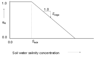
Salinity stress reduces the root water uptake and is related to the solute concentration in soil water. In SWAP, this effect is represented using the linear reduction function proposed by (Maas and Hoffman 1977). Figure 8.2 shows the reduction function of Maas and Hoffman (1977). The reduction of root water uptake (\(\alpha_{\text{rs}}\)) when the salt concentration exceeds a threshold value is linearly related to the salinity concentration:
\[ \alpha_{\text{rs}} = 1.0 - (c - S_{\text{max}}) S_{\text{slope}} \tag{8.26}\]
where \(c\) is the salinity concentration (mg cm-3), \(S_{\text{max}}\) is the salinity threshold value (mg cm-3), and \(S_{\text{slope}}\) is the decline of the root water uptake factor per unit increase of salinity concentration (cm3 mg-1).
8.6 Groundwater age
Soil moisture and groundwater age can be calculated as the time elapsed after entering the soil water domain described by the SWAP model. Following the method used by Goode (1996) and Lemieux and Sudicky (2010), the soil moisture age is governed by a convection-dispersion equation for an inert solute with an internal source of unit (1) strength:
\[ \frac{\partial A}{\partial t} = \frac{\partial}{\partial z} \left( D \frac{\partial A}{\partial z} \right) - v \frac{\partial A}{\partial z} + 1 \tag{8.27}\]
where \(A\) is the average age of water particles in a package of water (d).
The age of water entering the model boundaries is set to 0, irrespective of the boundary type. In soil profiles exposed to a constant upward flux at the bottom boundary, the age at the bottom equals zero and the distribution with depth shows a curved course.
The capabilities of the age module implemented in the SWAP model are illustrated in Figure 8.3. It shows the long-term averaged age distribution with depth for four classes of hydrological plots in the Dutch Nationwide STONE model (Groenendijk and Renaud 2013).
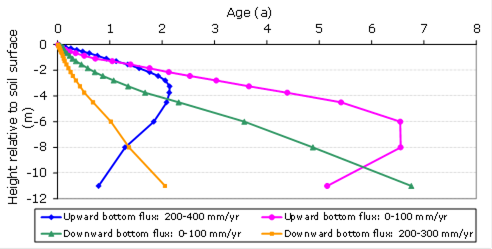
The age of soil water in the profiles with a relatively low leaching rate (0-100 mm yr-1) is higher than in the profiles with a relatively high leaching rate (200-300 mm yr-1) and the age in the profiles with a relatively low upward seepage (0-100 mm yr-1) is higher than in the profiles with a relatively high upward seepage rate (200-400 mm yr-1). The position of the maximum age in the profiles with upward seepage depends on the seepage flow rate and the layout of the drainage systems.
8.7 User instructions
Tip 8.1 lists the input data for solute transport, which are divided over the parts:
- Top and initial boundary condition
- Diffusion coefficient and solute uptake by roots
- Adsorption
- Decomposition
- Solute residence in the saturated zone
In general, the theory description in Section 8.2 – Section 8.5 in combination with the descriptions in the input file will be sufficient to guide the model user. A few additional remarks are appropriate at this place.
In case conservative solutes are simulated, like salts or non-reactive tracers, we need only to consider the transport processes convection, diffusion, dispersion, and passive uptake by plant roots.
At most field conditions we may neglect the effect of diffusion with respect to dispersion and therefore may specify \(D_{\text{dif}}\) = 0. The parameter dispersion length, \(L_{\text{dis}}\) (cm), depends on the scale over which the water flux and solute convection are averaged. Typical values of \(L_{\text{dis}}\) are 0.5 - 2.0 cm in packed laboratory columns and 5-20 cm in the field (Jury, Gardner, and Gardner 1991; Vanderborght and Vereecken 2007).
SWAP supports two methods to account for the residence time of solutes in the saturated zone. The first one by proper distribution of the lateral drainage flux over the saturated compartments (Chapter 4). In that case we may set swbr = 0 and specify the solute concentration in the groundwater as a boundary condition for upward flow (Tip 8.1). The second method has been described in this chapter and views the saturated zone as one mixed reservoir (Section 8.4). In that case we should set swbr = 1 and provide the effective transport properties of the saturated zone (Tip 8.1, Part 5).
The input data for salinity stress depend on the plant species and are listed in the crop input file. SWAP input data for the Maas and Hoffman reduction function are listed in Appendix K.
With the option swsolu = 2, simulation of soil moisture and groundwater age is activated. The model will automatically produce 2 output files: i) result.ageeffluent.csv and ii) result.ageprofile.csv with groundwater age (d) of respectively effluent and soil water.