6 Macropore flow

6.1 Introduction

In structured soils such as clay and peat, preferential flow occurs through large pores or macropores in the (un)saturated soil matrix. Macroporosity can be caused by shrinking and cracking of soil, by plant roots, by soil fauna, or by tillage operations. Macropores in SWAP are defined as pores with a diameter or width equal to or larger than 100 µm.

Due to the very rapid flow through macropores, water and solutes can reach to large depths within the soil profile rapidly after the onset of a rain shower, bypassing the capacity of the soil matrix for storage, adsorption, and transformation of potential pollutants. This process is known as ‘bypass flow’ or ‘short-circuiting’ (Hoogmoed and Bouma 1980). Because of the great impact of macropores on water flow and solute transport through the vadose zone, a concept has been implemented in SWAP for simulating preferential flow at the field scale.

Cracked clay soils reveal a large spatial variability of water contents and solute concentrations at given depth (Beven and Germann 1982; Bronswijk et al. 1995). Therefore, instead of trying to describe water flow and solute transport at each location, the field average behaviour may be easier to catch in a model. In order to make the model suitable for process and scenario analysis, concepts should be used that are generally applicable, thus physically based. Furthermore, model calibration requires a limited number of parameters, and preferably parameters that can be measured directly in the field. The description of macropore flow in SWAP has been developed taking into account these requirements.

In the SWAP model macropore water flow includes the following processes:

inflow of water into macropores at the top of the macropores;
vertical transport to deeper layers or the groundwater bypassing the soil matrix;
lateral infiltration into and exfiltration out of the soil matrix;
rapid drainage to drainage systems;
water storage in the macropores.

The simulation of these processes is based on the description of the macropore geometry as proposed by Hendriks et al. (1999). The description of this geometry that SWAP uses, is discussed in Section 6.2. In short, it consists of a main bypass flow domain (MB domain) and an internal catchment domain (IC domain). The MB domain forms one continuous network of interconnected macropores, whereas the IC domain consists of multiple subdomains with discontinuous and non-connected macropores ending at different depths. All domains may be subject to changes in pore volumes driven by the soil matrix head, reflecting swelling and shrinking of the soil.

Two different concepts of water flow within the macropores have been implemented in SWAP:

the ‘instantaneous bypass’ flow concept; it assumes water flowing into the macropore to be added to the water storage at the bottom of the macropores instantaneously. Lateral infiltration into the soil matrix of macropore water running rapidly downwards is neglected. This concept requires the use of both the MB and IC domains to allow for infiltration of macropore water along the soil profile;
the ‘kinematic wave’ flow concept; it models the flow of water in the unsaturated part of the macropore explicitly using a kinematic wave equation, allowing for exchange between macropore and matrix water over the entire macropore depth.

These water flow concepts are described in more detail in Section 6.4. Details on the exchange fluxes between the macropores and the top of the soil, the soil matrix or drainage systems is described in Section 6.3 and is independent of the flow concepts used. Finally, the sections Section 6.5 and Section 6.6 give some hints as to the numerical implementation and user instructions for SWAP simulations including macropore flow.

6.2 Macropore geometry

In SWAP the geometry of macropore structure is described by characterising the macropore volume according to three main properties:

Continuity: vertical continuity controls flow of water that is taken up at the soil surface to different depths in the profile and horizontal continuity controls exchange of water between macropores (Section 6.2.1);
Persistency: static macropore volume is permanent, while dynamic macropore volume (shrinkage cracks) depends on soil moisture status (Section 6.2.2);
Horizontal distribution: in the horizontal plane, macropore volume is distributed over cracks and holes. The shape of the horizontal cross section of the macropore volume has a large impact on the water exchange between macropore volume and soil matrix, and on rapid drainage (Section 6.2.3).

The concept provides a functional rather than a meticulous description of these macropore geometry properties. With a limited number of input parameters it determines a functional macropore bottom depth distribution, and magnitude and horizontal shape of the macropore volume as a function of depth.

A basic assumption in the concept is that property ‘persistency’ is not correlated with both other properties. ‘Persistency’ refers to volume and not to pore structure: static macropore volume and dynamic macropore volume form together the total macropore volume. Characterisation according to the other two properties applies to the total volume. The properties ‘continuity’ and ‘horizontal distribution’ are correlated: the horizontal macropore volume distribution as a function of depth depends on the macropore bottom depth distribution.

6.2.1 Continuity

With respect to vertical and horizontal continuity the macropores are divided into two classes that are integrated in two domains:

main bypass (MB) flow domain: the network of continuous, horizontal interconnected macropores;
internal catchment (IC) domain: discontinuous non-interconnected macropores, ending at different depths.

The MB domain represents the main system of continuous structural and shrinkage cracks, as well as root and worm holes. These macropores penetrate relatively deep into the soil profile and are assumed to be horizontally interconnected, for example in a network of structural and shrinkage cracks. In the MB domain water is transported relatively fast and deep into the profile bypassing the soil matrix. This may lead to short-circuiting between soil surface and groundwater, and rapid drainage to drains.

The IC domain represents macropores − cracks and holes − that are not interconnected and not connected to the MB domain, and that end at different depths in the profile. In this domain macropore inflow is entrapped at the bottom of individual macropores, resulting in forced infiltration of macropore water into the (mainly) unsaturated soil matrix at different, relatively shallow depths.

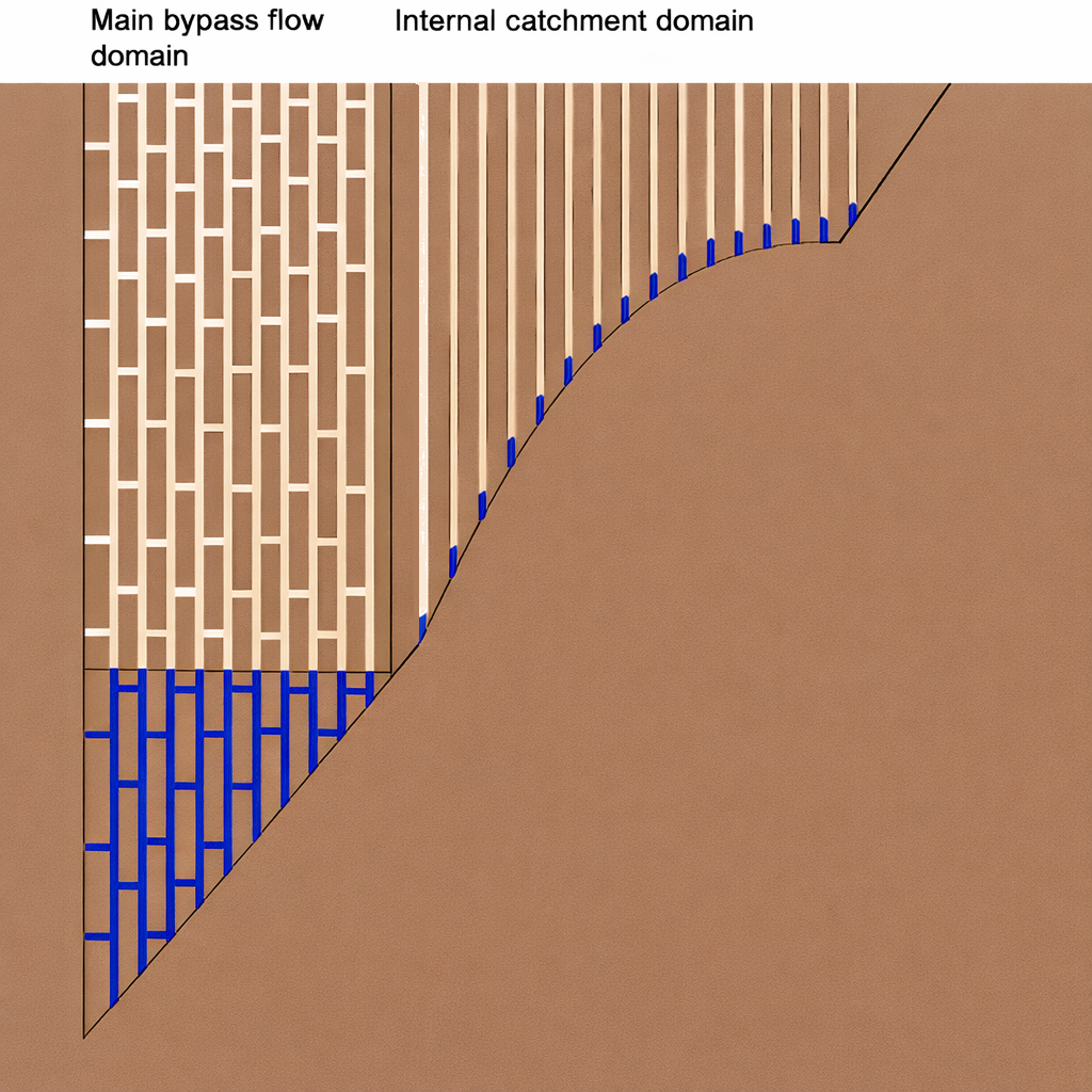
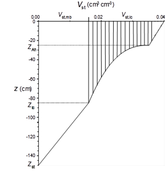
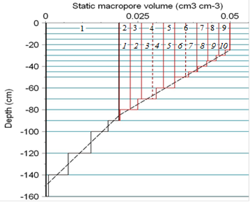
(a) Schematic representation of the two main domains: 1) Main bypass flow domain (MB): transporting water deep into the profile and possibly leading to rapid drainage, 2) Internal catchment domain (IC): infiltration of trapped water into the (mainly) unsaturated matrix at different depths.

Figure 6.1 (a) presents a conceptual visualisation of the two classes of macropores; Figure 6.1 (b) depicts a mathematical representation of the conceptual figure. It describes the static macropore volume fraction \(V_{st}\) (cm³ cm^-3) of the two domains, \(V_{st,mb}\) and \(V_{st,ic}\), as a function of depth. From these two volume fractions the partitioning of the static macropore volume over the two domains at any depth can be calculated. This partition as a function of depth is a crucial property of macropore geometry in the concept. It determines the distribution of macropore volume over both domains. It is expressed in the volumetric proportion \(P\) (-) of each domain:

\[ P_{mb} = \frac{V_{st,mb}}{V_{st,mb} + V_{st,ic}} \text{ and } P_{ic} = \frac{V_{st,ic}}{V_{st,mb} + V_{st,ic}}, \tag{6.1}\]

such that

\[ P_{mb} = 1 - P_{ic}. \tag{6.2}\]

Subscripts ‘mb’ and ‘ic’ refer to MB and IC domains, respectively. The IC volumetric proportion at the top of the macropores (an input parameter), \(P_{ic}^{tp}\) (-), determines the distribution over the two main domains at the top of the macropores (denoted by superscript \(tp\)). It is possible to consider only the MB domain, but it is not allowed to consider only the IC domain (\(0<P_{mb} \le 1\)).

In the concept, static macropore volume is not necessarily always present. But even in the absence of this volume, the volumetric proportions are required to partition the dynamic volume over the domains. Therefore, the calculation of the volumetric proportions as a function of depth is independent of the magnitude of the dynamic macropore volume. This calculation provides the ‘blueprint’ of the macropore domains. In order to visualize this ‘blueprint,’ it is more illustrative to show only the static macropore volume as is done in Figure 6.1 (b). Since the dynamic volume changes with time and depth, depending on shrinkage characteristics and soil moisture status that may differ at each depth, it would distort the image of the ‘blueprint.’

IC domain

It is assumed that the IC macropore volume consists of many individual small macropores that originate at the soil surface and functionally end at different depths. In this sense ‘functional’ implies that flow is blocked at the depth of ending of the macropores. Thus, the functional volume of IC macropores gradually declines to zero at depth \(Z_{ic}\) (cm), the bottom of the IC domain.

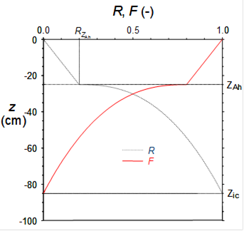
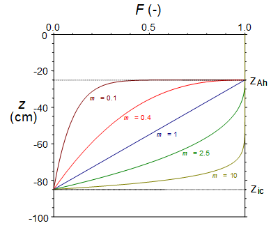
(a) Cumulative frequency distribution \(R\) of the depth \(z\) at which the functional IC macropores end and the fraction \(F\) of IC macropores that is functional at depth \(z\).

The fraction of functional macropores in the IC catchment is described by the function \(F\) (Figure 6.2). Its complementary function, \(R=1-F\), gives the cumulative frequency distribution of the depth \(z\) at which the functional IC macropores end. This is described with a power law function as

\[ R = \begin{cases} R_{Z_{Ah}} \frac{z}{Z_{Ah}} & \text{ for } 0 \ge z > Z_{Ah} \\ R_{Z_{Ah}} + (1 - R_{Z_{Ah}}) \left(\frac{Z_{Ah} - z}{Z_{Ah} - Z_{ic}}\right)^m & \text{ for } Z_{Ah} \ge z \ge Z_{ic} \\ 1 & \text{ for } z>Z_{ic} \end{cases}, \tag{6.3}\]

where the depths \(z\), \(Z_{Ah}\), and \(Z_{ic}\) (cm) are defined negative downwards, and the power \(m\) (-) is a shape factor. Power \(m\) > 1 describes shallow IC systems, while \(m\) < 1 describes deep IC systems; \(m\) = 1 (default) describes an intermediate system with a linear decline of functional IC macropores with depth. \(R_{Z_{Ah}}\) (-) is an optional parameter with which a linear increase of the \(R\)-curve over the thickness of the A-horizon, ending at depth \(Z_{Ah}\), can be described. Its default value is zero. Optionally, two more shape parameters are available to adjust the curves’ shape between \(Z_{Ah}\) and \(Z_{ic}\), detailed in Tip 6.1. Some examples of parameterisation are given in Appendix I. Note that \(Z_{Ah}\) may be set to field surface (its default), such that no distinction in macropore discription is made between the A-horizon and the soil below.

Tip 6.1: Optional shape parameters for the IC domain

Even more flexibility in the description of the IC domain can be provided with the optional input parameters for the symmetry point \(S_{pnt}\) (\(0<S_{pnt}\le 1\)) and the switch \(SW_{powm}\). Defining a symmetry point results in the introduction of an S-shaped curve. If also the switch \(SW_{powm}\) is set to 1, a double convex (\(m<1\)) or double concave (\(m>1\)) distribution is generated. Equation 6.3 is extended in case the symmetry point is introduced; the frequency distribution curve \(R\) is then calculated as

\[ R = \begin{cases} R_{Z_{Ah}} \frac{z}{Z_{Ah}} & \text{ for } 0 \ge z > Z_{Ah} \\ R_{Z_{Ah}} + {S_{pnt}}^{(1-m)}(1 - R_{Z_{Ah}}) \left(\frac{Z_{Ah} - z}{Z_{Ah} - Z_{ic}}\right)^m & \text{ for } Z_{Ah} \ge z \ge Z_{S_{pnt}} \\ 1-{(1-S_{pnt})}^{(1-m^*)}(1 - R_{Z_{Ah}}) \left(\frac{Z_{Ah} - z}{Z_{Ah} - Z_{ic}}\right)^{m^*} & \text{ for } Z_{S_{pnt}} \ge z \ge Z_{ic} \\ 1 & \text{ for } z>Z_{ic} \end{cases}, \tag{6.4}\]

with power

\[ m^*= \begin{cases} m &\text{ if } SW_{powm} = 0 \\ 1/m&\text{ if } SW_{powm} = 1 \end{cases} \tag{6.5}\]

and the depth at which the symmetry point is situated given as

\[ Z_{S_{pnt}}=Z_{Ah}-S_{pnt}(Z_{Ah}-Z_{IC}). \tag{6.6}\]

The volumetric proportion of IC macropore volume as a function of depth can be written in terms of the constant \(P_{ic}^{tp}\) and the frequency distribution \(R\), as

\[ P_{ic} = \begin{cases} \frac{1-R}{\frac{1}{P_{ic}^{tp}} - R} & \text{ for } 0 \ge z > Z_{ic} \text{ and } 0 < P_{ic}^{tp} < 1 \\ 0 & \text{ for } z \le Z_{ic} \text{ or }P_{ic}^{tp} = 0 \end{cases}. \tag{6.7}\]

The volumetric proportion of MB macropore volume as a function of depth is calculated from function \(P_{ic}\) with Equation 6.2. This results in a proportion \(P_{mb}\) of 1 for depths below \(Z_{ic}\) where IC macropore volume is absent and all macropore volume is MB volume.

Constructing the macropore subdomains

To obtain the required resolution in IC macropores, the IC domain is divided into \(n_{sd}\) subdomains. If option \(R_{Z_{AH}} > 0\) is chosen, an extra Ah-subdomain \(k = n_{sd} + 1\) is created. This partition represents the horizontal discretisation of the macropore system. The IC volume at soil surface, minus the \(R_{Z_{AH}}\) volume, is equally distributed over the \(n_{sd}\) subdomains. The volumetric proportion \(P_{k}\) of any subdomain \(k\) in the IC domain as a function of \(z\) is calculated according to:

\[ P_{k} = \begin{cases} \frac{1}{\frac{1}{P_{ic}^{tp}} - R} \frac{1 - R_{Z_{Ah}}}{n_{sd}} & \text{for} \quad 0 \ge z > z_{k+1} \\ \frac{1-R - \frac{k-1}{n_{sd}} (1 - R_{Z_{Ah}})}{\frac{1}{P_{ic}^{tp}} - R} & \text{for} \quad z_{k+1} \ge z > z_{k} \\ 0 & \text{for} \quad z \le z_{k} \\ \end{cases}, \tag{6.8}\]

where \(k = 1\) is the deepest and \(k = n_{sd}\) the shallowest subdomain (respectively left and right in Figure 6.1 (b)), and \(z_{k}\) is the depth at which subdomain \(k\) ends:

\[ z_{k} = Z_{Ah} - (Z_{Ah} - Z_{ic}) \left(1 - \frac{k-1}{n_{sd}}\right)^{\frac{1}{m}}. \tag{6.9}\]

Because the MB domain is always present, though sometimes with very low proportion, the total number of domains \(n_{dm} = n_{sd} + 1\). In case of \(R_{Z_{AH}} > 0\), \(n_{dm} = n_{sd} + 2\). All domains are numbered from \(j = 1\) to \(n_{dm}\) with the MB domain being the first domain \(j = 1\) and the deepest IC domain the second \(j = 2\).

In the model, the vertical coordinate \(z\) is partitioned into discrete model compartments \(i\) with thickness \(\Delta z,i\) (cm) between \(z_{b,i}\) and \(z_{t,i}\) at the bottom and top of the compartment, respectively. For each compartment a discrete macropore volume per domain is required. Volumetric proportion \(P_{j,i}\) for each combination of domain \(j\) and compartment \(i\) is obtained by integration of \(P_{mb}\) and \(P_{k}\) as a function of \(z\) over the compartment thickness and dividing by \(\Delta z_i\):

\[ P_{1,i} = \frac{\int_{z_{b,i}}^{z_{t,i}} P_{mb} \, dz}{\Delta z_i} \quad \text{and} \quad P_{j,i} = \frac{\int_{z_{b,i}}^{z_{t,i}} P_{k=j-1} \, dz}{\Delta z_i} \quad \text{for} \quad 2 \le j \le n_{dm}. \tag{6.10}\]

Per domain the macropore volume is vertically interconnected over the soil compartments. IC subdomains that end in the same model compartment, are functionally equal and therefore are lumped for all compartments \(i = 1\) to \(i_{bot_j}\) (compartment number that contains bottom of domain \(j\)).

For each lumped domain \(n_{dm}\) is reduced with 1. In this way, the resolution of the horizontal discretisation in terms of \(n_{dm}\) is determined by \(n_{sd}\), the thickness of compartments and the shape of curve \(R\): the combination of large \(n_{sd}\), small \(\Delta z\)’s and a linear \(R\)-curve (\(m = 1\)) yields the largest \(n_{dm}\). An example of the lumping of macropore geometry in the IC subdomains is given in Figure 6.3.

Figure 6.3: Example of a combination of horizontal (red lines) and vertical (blue lines) discretisation: number of IC sub-domains given as input \(n_{sd}\) = 10 (italic numbers) while the resulting total number of domains \(n_{dm}\) = 9 (regular numbers). Former subdomains 3 and 4 are lumped to obtain present domain 4, and former subdomains 6 and 7 are lumped to obtain present domain 6 as they end in the same vertical model compartment. Parameters used: \(V_{st,0}\) = 0.05 cm³ cm^-3, \(P_{ic,0}\) = 0.6, \(m\) = 1, \(R_{Z_{Ah}}\) = 0, \(Z_{AH}\) = −20 cm, \(Z_{ic}\) =−85 cm, \(Z_{st}\) =−150 cm.

Cover layer

A situation may exists where macropores are present in the sub soil, but absent in the top soil. An example of a SWAP application for situation with a cover layer without macropores is described in (Berg et al. 2022). Setting \(Z_{tp} < 0\) (cm) introduces such a cover layer, while overriding the value of \(Z_{Ah}\), such that the A-horizon ends at depth \(Z_{tp}\). In addition, \(R_{Z_{Ah}}\) is set to 0. In case a cover layer is considered, the same calculation procedure with regard to macropore continuity holds as described above, except that for \(0\le z < Z_{Tp}\), all domain proportions \(P_{k}\) and \(P_{mb}\) are set to 0.

6.2.2 Persistency

With respect to persistency, the macropore volume of each of the domains consists of:

static macropore volume, expressed as volume fraction \(V_{st}\) (cm³ cm^-3), representing macropores that are permanently present. The static volume as a function of depth is constant in time;
dynamic macropore volume, expressed as volume fraction \(V_{dy}\) (cm³ cm^-3), i.e., shrinkage cracks. The dynamic volume as a function of depth is not constant in time.

The dynamic shrinkage volume is added to the static volume, if present, and in this way enlarges the total macropore volume (Figure 6.4). The total macropore volume fraction \(V_{mp}\) (cm³ cm^-3) is distributed over the two domains according to their volumetric proportion:

\[ V_{mp} = V_{st} + V_{dy}, \tag{6.11}\]

\[ V_{mb} = P_{mb} V_{mp} = P_{mb} (V_{st} + V_{dy}) = V_{st,mb} + P_{mb} V_{dy}, \tag{6.12}\]

\[ V_{ic} = P_{ic} V_{mp} = P_{ic} (V_{st} + V_{dy}) = V_{st,ic} + P_{ic} V_{dy}. \tag{6.13}\]

This implies that below depth \(Z_{ic}\) all dynamic volume is part of the MB domain, and below depth \(Z_{st}\), only dynamic volume may occur.

Static macropore volume

The static macropore volume consists of structural shrinkage cracks, biopores (e.g., worm and root holes), and macropores that originate from tillage operations. Contrary to dynamic macropore volume, it is independent of the soil moisture status. The volume fraction of static macropores per domain as a function of depth \(z\) is described with the constant \(P_{ic}^{tp}\), the function \(R\) (Equation 6.3), and the two additional input parameters \(V_{st}^{tp}\) (-), describing the volume fraction of static macropores at the top of the macropores, and \(Z_{st}\) (cm), signifying the maximum depth of static macropores.

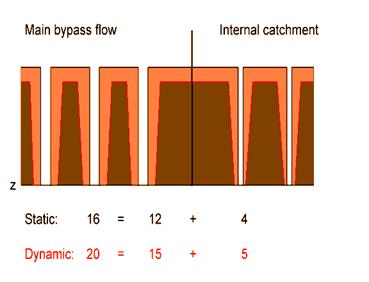
Figure 6.4: Partitioning of static and dynamic macropore volume over the two macropore domains according to the volumetric proportions of the domains (\(P_{ic}\) = 0.25): ratio between MB and IC domains is equal for static and dynamic macropore volume. White areas represent static and light areas dynamic macropore volume. Dark colour is the soil matrix. Numbers are imaginary macropore volumes meaning: Total = Main Bypass + Internal Catchment.

In general (all \(V\) in cm³ cm^-3):

\[ V_{st} = V_{st,mb} + V_{st,ic} \text{ and thus } V_{st}^{tp} = V_{st,mb}^{tp} + V_{st,ic}^{tp}, \tag{6.14}\]

where the volumes at the top of the macropore are given as

\[ V_{st,ic}^{tp} = P_{ic}^{tp} V_{st}^{tp} \text{ and } V_{st,mb}^{tp} = (1 - P_{ic}^{tp}) V_{st^{tp}}. \tag{6.15}\]

The static macropore volume fraction of the MB domain as a function of depth is calculated as

\[ V_{st,mb} = \begin{cases} V_{st,mb}^{tp} & \text{ for } 0 \ge z > Z_{ic} \\ V_{st,mb}^{tp} \left(\frac{z - Z_{st}}{Z_{ic} - Z_{st}}\right)^{m_{mb}} & \text{ for } Z_{ic} \ge z > Z_{st} \\ 0 & \text{ for } z \le Z_{st} \\ \end{cases}, \tag{6.16}\]

where power \(m_{mb}\) introduces an option for a non-linear change in MB volume below \(Z_{ic}\). It is calculated as

\[ m_{mb}=\frac{\log(0.5)}{\log\left(\frac{Z_{mb50}-Z_{st}}{Z_{ic}-Z_{st}}\right)}, \tag{6.17}\]

where \(Z_{mb50}\) (cm) (with \(Z_{ic}>Z_{mb50}>Z_{st}\)) is an optional input parameter stating at which depth the MB volume fraction is 50% of \(V_{st,mb}^{tp}\). A default is given as \(Z_{mb50}=(Z_{ic}+Z_{st})/2\), resulting in a linear decline of the static MB volume below \(Z_{ic}\).

The static macropore volume fraction of the IC domain as a function of depth is given as

\[ V_{st,ic} = \begin{cases} (1-R) V_{st,ic}^{tp} & \text{ for } 0 \ge z > Z_{ic} \\ 0 & \text{ for } z \le Z_{ic} \\ \end{cases}. \tag{6.18}\]

Dynamic macropore volume

The dynamic macropore volume originates from the shrinking of the soil matrix due to soil moisture loss. In general, this process is restricted to soils that contain substantial amounts (> 10-15 mass-%) of clay minerals (except kaolonite) and/or organic matter. Mostly, the shrinkage volume occurs as shrinkage cracks. Shrinkage of the matrix may also enlarge cylinder-shaped macropores. In SWAP it is assumed that shrinkage enlarges the present permanent macropore volume and consequently the shrinkage volume is added to the static volume (Equation 6.3).

Soil matrix shrinkage occurs in both the vertical and horizontal direction. Vertical shrinkage leads to soil surface subsidence, horizontal shrinkage to dynamic macropore volume. The dynamic volume is calculated from overall and vertical shrinkage as

\[ V_{dy} = V_{sh} - V_{su}, \tag{6.19}\]

where \(V_{sh}\), \(V_{dy}\) and \(V_{su}\) (all in cm³ cm^-3) are the volume fraction of overall matrix shrinkage, the dynamic macropore volume fraction, and the subsidence volume fraction, respectively.

In the present version of SWAP the vertical shrinkage does not affect the vertical coordinate system of SWAP. This approach avoids numerical problems that may result from solving Richards equation for a dynamic vertical coordinate. We assume that at the field scale the effects of ignoring changes of the soil matrix in vertical direction are small as compared to effects of uncertainties in other processes and input parameters.

However, the approach of ignoring vertical changes in soil matrix does affect the calculation of the dynamic macropore volume. This volume is corrected for the vertical shrinkage according to

\[ V_{dy} = (1 - V_{st}) \frac{V_{sh} - V_{su}}{1 - V_{su}}. \tag{6.20}\]

In this way the ratio between \(V_{dy}\) on one hand, and the matrix volume fraction and the static macropore volume fraction \(V_{st}\) on the other hand is consistent. The first term is the horizontal area fraction of the matrix, which accounts for the static macropore volume.

The vertical shrinkage component is determined from the overall matrix shrinkage as (Bronswijk 1988)

\[ V_{su} = 1 - (1 - V_{sh})^{1/r_s}, \tag{6.21}\]

where exponent \(r_s\) (-) is the geometry factor (Rijniersce 1983). In case of three-dimensional isotropic shrinkage, \(r_s = 3\). When cracking dominates subsidence \(r_s > 3\), when subsidence dominates cracking \(1 < r_s < 3\). In case of subsidence only, \(r_s = 1\). The geometry factor is an input parameter.

Shrinking and swelling behaviour in the field may deviate from that in the laboratory because of overburden pressure of overlaying soil layers in the field. This may result in delayed horizontal shrinkage in favour of vertical shrinkage. To account for this process, a threshold moisture content \(\theta_{crack}\) is introduced. For moisture contents \(\theta \geq \theta_{crack}\) all shrinkage is vertical and for \(\theta < \theta_{crack}\) shrinkage is vertical and horizontal according to geometry factor \(r_s\). This concept does not apply to swelling: shrinkage cracks are not closed before saturation. \(\theta_{crack}\) is an input parameter.

The matrix shrinkage volume fraction \(V_{sh}\) is a function of volumetric moisture content and shrinkage characteristic. A shrinkage characteristic describes the relationship between soil volume and soil moisture content. Many forms of shrinkage characteristics exist. A very convenient one is the characteristic that takes the constant volume fraction of the solid soil fraction \(V_{sol}\) as reference for all variable volume fractions and expresses the soil matrix volume fraction \(V_{mt}\) in terms of pore volume fraction \(V_{por}\) relative to \(V_{sol}\) (Bronswijk 1988) (all \(V\) in cm³ cm^-3):

\[ V_{mt} = V_{sol} + V_{por} = (1 + e)V_{sol}, \tag{6.22}\]

where \(e\) (cm³ cm^-3) is the void ratio

\[ e = \frac{V_{por}}{V_{sol}}. \tag{6.23}\]

The shrinkage volume fraction \(V_{sh}\) is equal to the fraction of volume loss of the matrix that in its turn equals the fraction loss of pore volume. The latter is expressed in terms of \(e\) and \(V_{sol}\) as

\[ V_{sh} = -\Delta V_{mt} = -\Delta V_{por} = -\Delta e V_{sol} = -(e - e_s)V_{sol}, \tag{6.24}\]

where \(e_s\) is the void ratio at saturation.

The shrinkage characteristic expresses the variable \(e\) as a function of the moisture ratio:

\[ e = f(\vartheta), \tag{6.25}\]

where the moisture ratio \(\vartheta\) (cm³ cm^-3) is defined as

\[ \vartheta = \frac{\theta}{V_{sol}} = \frac{\theta}{1 - \theta_s}, \tag{6.26}\]

with \(\theta\) the actual water volume fraction. Volume fraction of solids \(V_{sol}\) (cm³ cm^-3) equals \(1 - \theta_s\) (\(\theta_s = \theta\) at saturation).

The exact form of the shrinkage characteristic depends on soil texture - in terms of content and nature of clay minerals - and organic matter. Shrinkage characteristics of clay and organic soils (peat and peaty soils) differ strongly (Figure 6.5), and are considered separately in the following two sections.

Figure 6.5: Typical shrinkage characteristic of (A): clay (modified after Bronswijk (1988)) and (B): peat (after Hendriks (2004)), expressed as void ratio \(e\) as a function of moisture ratio \(\vartheta\), showing the three shrinkage stages. Black dots in B. are measurements while solid line is fit with Equation 6.29

Shrinkage characteristic of clay and clayey soils

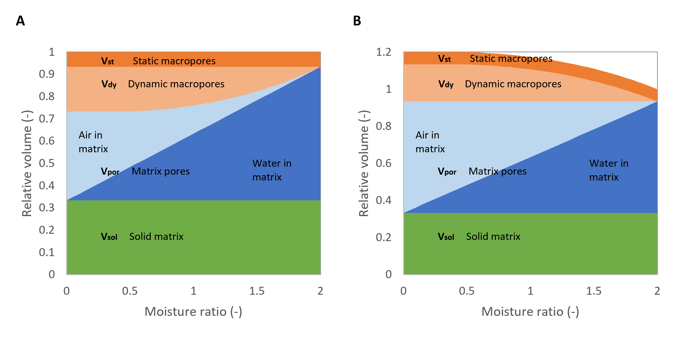
Figure 6.5 A shows a typical shrinkage characteristic of a clay soil. Three stages can be distinguished (Stroosnijder 1975; Bronswijk 1988):

normal shrinkage: volume decrease of clay aggregates is equal to moisture loss. The aggregates remain fully saturated;
residual shrinkage: upon drying the volume of the aggregates still decreases, but moisture loss is greater than volume decrease. Air enters the pores of the aggregates;
zero shrinkage: soil particles reach their most dense configuration. Upon further moisture extraction, the volume of the aggregates remains constant. Moisture loss equals air volume increase of the aggregates. Rigid soils, like sands, only show this stage.

A fourth shrinkage stage that precedes normal shrinkage may be recognized: structural shrinkage. When saturated soils dry, large water-filled pores may be emptied. As a result, aggregates can get a somewhat denser packing. Overall, the volume changes in this stage are negligible, but water losses can be considerable. In SWAP, structural shrinkage is explicitly accounted for in the form of the static macropores, e.g. structural shrinkage cracks. The first three real shrinkage stages are computed as a function of moisture content with the equation of Kim (1992):

\[ e = \alpha_K \exp(-\beta_K \vartheta) + \gamma_K \vartheta \ \text{ for } \ 0 < \vartheta < \vartheta_s, \tag{6.27}\]

where

\[ \vartheta_s = \frac{\theta_s}{1 - \theta_s}. \tag{6.28}\]

The term \(\alpha_K\) (cm³ cm^-3) equals \(e_0\) (the void ratio at \(\vartheta = \theta = 0\)), \(\beta_K\) and \(\gamma_K\) are dimensionless fitting parameters and \(\vartheta_s\) is the void ratio at saturation. Using Equation 6.27, \(e\) may become smaller than \(e_0\), in which case the model sets \(e\) to \(e_0\) (zero shrinkage).

Shrinkage characteristic of peat and peaty soils

According to Hendriks (2004), for peat soils three shrinkage stages can be distinguished as well (Figure 6.5 B):

near-normal shrinkage: volume reduction equals nearly moisture loss, little air enters the pores and the peat matrix remains close to saturation;
subnormal shrinkage: upon drying moisture loss exceeds volume reduction, air enters the relatively large pores while the small pores in the organic fibres, that form the ‘skeleton’ around the larger pores, remain water-filled;
supernormal shrinkage: volume reduction exceeds moisture loss, small pores are emptied and the skeleton collapses, so that air is driven out of the larger pores and the matrix reaches its final, smallest volume when the moisture content is zero.

The equation for the shrinkage curve of peat and peaty soils reads (Hendriks (2004))

\[ e = \begin{cases} e_t \left(1 + P_H \frac{(\vartheta_t^{\alpha_H} \exp(-\beta_H \vartheta_t) - \exp(-\beta_H))}{\vartheta_{t,P}^{\alpha_H} (\exp(-\alpha_H) - \exp(-\beta_H))}\right) & \text{for} \ 0 < \vartheta < \vartheta_a \\ e_t & \text{for} \ \vartheta_a \leq \vartheta < \vartheta_s \end{cases}, \tag{6.29}\]

with

\[ \begin{align} e_t & = e_0 + (e_s - e_0) \frac{\vartheta}{\vartheta_s} ;\\ e_s & = \vartheta_s = \frac{\theta_s}{1 - \theta_s} ;\\ \vartheta_t & = \frac{\vartheta}{\vartheta_a} ;\\ \vartheta_{t,P} & = \frac{\alpha_H}{\beta_H} \quad \text{for} \ 0 < \alpha_H < \beta_H. \end{align} \tag{6.30}\]

Here, \(\vartheta_a\) is the moisture ratio at the transition of the near-normal shrinkage stage to the subnormal shrinkage stage, when air entry increases substantially. \(\alpha_H\), \(\beta_H\) and \(P_H\) are dimensionless fitting parameters.

Implications of macropores for the soil matrix

The presence of a macropore volume in addition to the soil matrix has implications on the matrix volume and the amount of water in the soil (Figure 6.6 A). Variable \(\theta\) describes the relative water content in the soil matrix as the volume water divided by the volume of soil matrix, thus excluding the static macropore volume. The water volume in the soil matrix at a given depth relative to the total volume (soil matrix plus macropore), \(V_{wat,mt}\) (cm³ cm^-3), is therefore given as

\[ V_{wat,mt} = \theta V_{mt} = \theta (1-V_{st}), \tag{6.31}\]

where \(V_{mt}\) (cm³ cm^-3) denotes the volume of the soil matrix relative to the total volume at a given depth. Parameters as the hydraulic conductivity of the soil matrix are reduced by the relative matrix volume in a similar way.

Strictly speaking, the dynamic nature of the macropores should also impact the soil matrix. Figure 6.6 A shows the conceptual volume partitioning as function of the moisture ratio. The total volume should always be equal to 1. With a constant static macropore volume (\(V_{st}\)) and constant volume of solid soil particles (\(V_{sol}\) ), the increase in dynamic volume (\(V_{dy}\)) with decreasing soil moisture content should result in a decrease in matrix pore volume (\(V_{por}\)) as indicated by the declining blue area in Figure 6.6 A with decreasing moisture content. However, this relation has not been implemented in SWAP as the matrix porosity is assumed constant. This implies that the amount of air in the soil matrix at a given moisture ratio is overestimated and that the relative saturation of the soil matrix is underestimated (Figure 6.6 B). These effects are partly compensated for by the fact that the soil moisture retention characteristics in SWAP are defined relative to the original volume of the soil matrix as well.

Figure 6.6: (A) Theoretical volume partitioning of a clay soil, as function of moisture ratio. Orange colors denote macropore volume, with a constant static (dark) and variable dynamic (light) volume. Blue colors indicate matrix pore volume, either filled with water (dark) or air (light). The constant solid matrix volume is indicated by green. (B) The actual volume partitioning as implemented in SWAP, with a constant matrix volume.

6.2.3 Horizontal distribution

In the horizontal plane in the field, macropore volume is distributed over different forms of macropores: from holes with a diameter of 100 \(\mu\)m to several centimetres wide, several decimetres long cracks. This distribution determines the functional horizontal shape of the macropores, which forms the basis of the calculation of several important parameters:

two parameters that affect lateral water exchange between macropores and soil matrix:
1. the vertical area of macropore walls per unit of volume, and
2. the distance from macropore wall to centre of matrix polygons;
the lateral hydraulic conductivity of cracks in case of rapid drainage.

For simplicity and input parameter limitation, cracks and hole-shaped macropores are not explicitly distinguished. Instead, they are implicit in an effective functional horizontal macropore shape that is described by an effective matrix polygon diameter \(d_{pol}\) (cm) as a function of depth.

Assuming effective regular soil matrix polygons, the effective vertical area of macropore walls per unit of volume \(A^*_{wall}\) (cm² cm^-3) is equal to the quotient of the perimeter divided by the area of the polygons. For all even-sided regular polygons, from square to circle, this quotient equals (see Appendix I for derivation)

\[ A^*_{wall} = \frac{4}{d_{pol}}. \tag{6.32}\]

The effective horizontal distance \(x_{pol}\) (cm) from macropore wall to matrix polygon centre is taken equal to

\[ x_{pol} = \frac{1}{2} d_{pol}. \tag{6.33}\]

The effect of horizontal macropore shape on rapid drainage is expressed through the effect on the lateral hydraulic conductivity of cracks which depends on the effective crack width \(w_{cr}\) (cm) (see Section 6.3.5). This width is calculated from the effective polygon diameter and the volume fraction \(V_{mb}\) of macropores in the MB domain (see Appendix I for derivation) as

\[ w_{cr} = \frac{4}{d_{pol}} \frac{V_{mb}}{1 - V_{mb}}. \tag{6.34}\]

It is assumed that the effective diameter \(d_{pol}\) of the soil polygons is a function of depth with its minimum value at the soil surface where macropore density is maximal and consequently distances between macropores are relatively small, and its maximum value deeper in the profile where macropore density is minimal. \(d_{pol}\) as a function of depth is determined from a maximum \(d_{p,max}\) and minimum \(d_{p,min}\) polygon diameter, both input parameters, and the relative macropore density \(M\) (-) as a function of depth according to

\[ d_{pol} = d_{p,min} + (d_{p,max} - d_{p,min})(1 - M), \tag{6.35}\]

where \(M\) is calculated as

\[ M= \begin{cases} \frac{V_{st}}{V_{st}^{tp}} & \text{ if } \ V_{st}^{tp} > 0 \\ \frac{P_{ic}}{P_{ic}^{tp}} & \text{ if } \ V_{st}^{tp} = 0 \ \text{and} \ P_{ic}^{tp} > 0 \\ \max(0, 1 - \frac{z}{Z_{dpmax}}) & \text{ if } \ V_{st}^{tp} = 0 \ \text{and} \ P_{ic}^{tp} = 0 \end{cases}. \tag{6.36}\]

If no static macropore volume and no IC domain are present (the third case in Equation 6.36), \(M\) is defined as a function of depth with \(Z_{dpmax}\) (cm) an input parameter denoting the depth below which \(d_{pol}\) equals \(d_{p,max}\).

6.3 Macropore water exchange

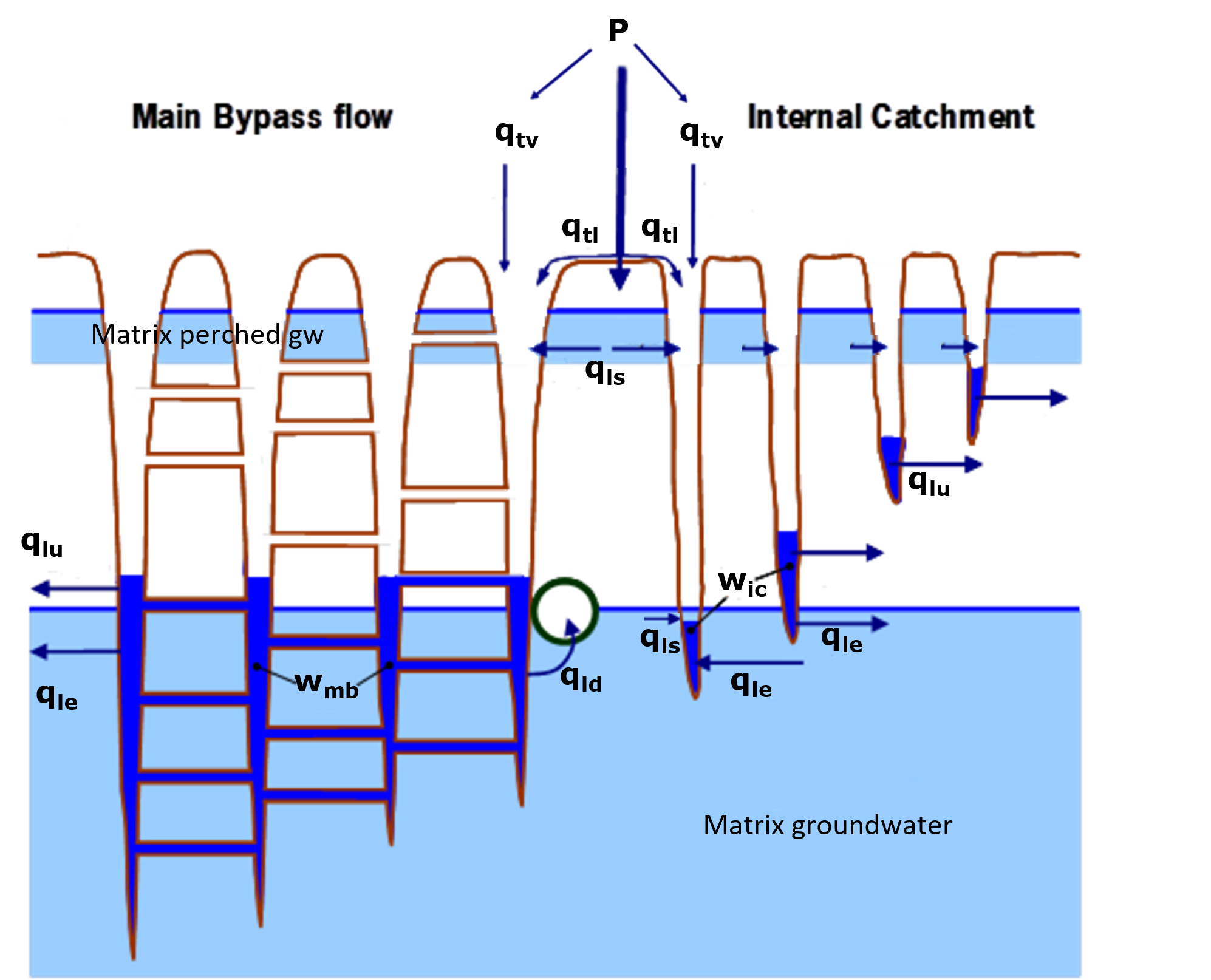
In SWAP, the exchange fluxes between the macropores and the top of the soil, the soil matrix and drainage systems include (Figure 6.7):

infiltration of water into macropores at the top of the macropore. This can include water falling vertically on top of the macropores \(q_{tv}\) (cm d^-1), lateral inflow by overland flow (runoff) into the macropores \(q_{tl}\) (cm d^-1) or, in case of a cover layer, water infiltrating vertically into the macropore at the bottom of the cover layer (\(q_{tv}\));
lateral flow from the macropore into the unsaturated soil matrix \(q_{lu}\) (cm d^-1);
lateral exchange between the saturated macropore and saturated matrix \(q_{le}\) (cm d^-1);
lateral flow from the saturated matrix to the unsaturated macropore \(q_{ls}\) (cm d^-1);
rapid drainage to drainage systems \(q_{ld}\) (cm d^-1).

All lateral fluxes are considered per macropore subdomain (if relevant), as they depend on the moisture status within each subdomain.

Figure 6.7: Schematic representation of the soil profile with soil matrix, drain, groundwater, perched groundwater, macropores in MB and IC domains, and the various macropore water balance terms. Mark that the saturated lateral exchange flux \(q_{le}\) can occur in two directions. See text for explanation of terms.

6.3.1 Inflow at the top of macropores

Macropores starting at the soil surface

In a situation without a non-macroporous cover layer the inflow of water into macropores at the soil surface consists of direct, vertical inflow into the top of the macropore (\(q_{tv}\)) and inflow into the top of the macropores from lateral flow over the soil surface (\(q_{tl}\)).

The rate \(q_{tv}\) (cm d^-1) of precipitation, irrigation and snowmelt water routed directly into the macropores beginning at the soil surface at a given precipitation/irrigation/snowmelt intensity \(I\) (cm d^-1) is calculated as

\[ q_{tv} = A_{Z_{cr}} I, \tag{6.37}\]

where \(A_{Z_{cr}}\) (cm² cm^-2) is the horizontal macropore area fraction at depth \(Z_{cr}\). The input parameter \(Z_{cr}\) (cm) is introduced for numerical reasons, because thin compartments in the top soil can result in rapidly changing moisture conditions in the top soil.

In case of a snowpack on top of the soil surface, it is assumed that the macropores are sealed off from the atmosphere and consequently \(q_{tv} = 0\), except when snowmelt occurs.

Infiltration rate term \(q_{tl}\) (cm d^-1) occurs when the head boundary condition holds for the top boundary of the soil matrix (see Equation 4.1 and Appendix E). In that case the water balance of the ponding layer is calculated, which includes \(q_{tl}\). Ponding occurs when the total of precipitation, irrigation, snow melt, runon and inundation intensity exceeds soil matrix infiltration capacity. Runoff into the macropores is then described in the same form as used for regular runoff to surface water or adjacent fields (Section 4.1) to allow for similar incorporation into the numerical solution of the top boundary (Appendix E):

\[ q_{tl} = \frac{h^{tp}}{\gamma_{tl}}, \tag{6.38}\]

where \(h^{tp}\) (cm) is the pressure head at the soil surface that equals the ponding height and \(\gamma_{tl}\) (d) is the resistance for macropore inflow at the soil surface. The macropore inflow resistance is estimated from the maximum ponding height \(h_{max}^{tp}\) (cm) assuming no runoff (neither into macropores nor regular), and the vertical hydraulic conductivity of the macropores at soil surface \(K_{v,mp}\) (cm d^-1). The latter is derived as a function of effective macropore width at soil surface from a theoretical slit model presented by Bouma and Anderson (1973):

\[ \gamma_{tl}=\frac{h_{max}^{tp}}{K_{v,mp}} \quad \text{ with } \quad K_{v,mp}=14.4* 10^8 \frac{(d_{pol}^{tp}(1-\sqrt{1-A_{Z_{cr}}}))^3}{d_{pol}^{tp}} \tag{6.39}\]

It can be seen that even the lower limit of macropore width (100 \(\mu\)m) yields large conductivities in the order of 100-1000 (cm d^-1) and consequently very low inflow resistances of 0.001-0.01 d. This implies that ponding water is routed preferentially into macropores. To account for the micro relief at the soil surface, mostly a threshold value for ponding height is used that must be exceeded before regular runoff starts. It is assumed that this does not apply to runoff into macropores, because it is very likely that micro depressions at the soil surface are connected to macropores. As a consequence, runoff into macropores is favoured over regular runoff and thus \(\gamma_{tl}\) is not a very sensitive variable.

The distribution of \(q_{tl}\) over the subdomains is according to the domain proportions at the soil surface \(P^{tp}\) (Equation 6.10).

Macropores starting below a cover layer

In a simulation with a cover layer, inflow into the top of the macropores is not a consequence of inflow of precipitation or overland flow. Rather, direct inflow of water may occur if the bottom of the cover layer is saturated as described in Berg et al. (2022):

\[ q_{tv}=\begin{cases} 0 & \text{ if } h_{z=Z_{tp}} < 0 \\ -\omega_{cl} K_s \left[ \frac{\partial (h+z)}{\partial z} \right]_{z=Z_{tp}} & \text{ if } h_{z=Z_{tp}} \ge 0 \end{cases}. \tag{6.40}\]

Here, the geometry coefficient \(\omega_{cl}\) (-) represents the influence of flow contraction at the interface of the covering layer and the macroporous layer. It is derived from an analogy with the flow of water in soil to tile drains, and accounts for vertical, horizontal and radial flow components, in analogy of Ernst (1962):

\[ \omega_{cl}=\frac{1}{1+\frac{d_{pol}}{\pi \frac{1}{2} \Delta z_{z=Z_{tp}}}\ln \left( \frac{d_{pol}}{\pi \frac{1}{2} w_{cr}} \right)+\frac{d_{pol}^2}{6\Delta z_{z=Z_{tp}}^2}}, \tag{6.41}\]

where \(d_{pol}\) and \(w_{cr}\) are given by Equation 6.35 and Equation 6.34, respectively, immediately below \(z=Z_{tp}\). A derivation of Equation 6.41 is given in Berg et al. (2022).

Lateral inflow into the top of the macropore, \(q_{tl}\), is set to zero in case of a cover layer. The distribution of \(q_{tv}\) over the macropore domains is according to the distributions immediately below \(z=Z_{tp}\).

6.3.2 Lateral flow into the unsaturated soil matrix

Two lateral infiltration mechanisms for infiltration of water in the unsaturated soil matrix can be relevant:

absorption of macropore water when capillary forces dominate;
Darcy flow due to a pressure head gradient from the macropore wall to the centre of the effective matrix polygon.

Absorption is the dominant mechanism at low soil moisture contents. It will be negligible under wet conditions even when there is a large pressure head gradient. In the latter case Darcy flow will be dominant. Darcy flow is very small under dry conditions because of very low hydraulic conductivities. Therefore, for each situation the flow rates of both infiltration mechanisms are calculated and the unsaturated infiltration flux is set equal to the largest of these two rates. The use of the Darcy absorption flux is optional.

Two alternative absorption mechanisms are implemented in SWAP. The first concept describes lateral absorption using Philip’s sorptivity (Philip 1957). The second uses a diffusion approach, similar as in MACRO (Larsbo and Jarvis 2003). Either one of the concepts needs to be chosen. It is advised to use the diffusion approach when considering the kinematic wave flow concept, due to the longer contact times between macropore water and the matrix wall.

Sorptivity

Lateral absorption can be described with Philip’s sorptivity (Philip 1957) as

\[ q_{lu,ab}^* = A_{wall,mtx}^* S_P \frac{\sqrt{t_2}-\sqrt{t_1}}{t_2-t_1} = \frac{4\sqrt{1-V_{mp}}}{d_{pol}}S_P\frac{\sqrt{t_2}-\sqrt{t_1}}{t_2-t_1}, \tag{6.42}\]

where \(q_{lu,ab}^*\) is the lateral absorption rate per unit of depth (cm cm^-1 d^-1) for a given subdomain \(j\) over time interval \(t_1 \rightarrow t_2\) (d), where \(t_1\) and \(t_2\) are the total time that has passsed since \(t = t_0\), the time of first contact between macropore water with the matrix. The term \(S_P\) is Philip’s sorptivity (cm d^-0.5), and the meaning of \(A_{wall,mtx}^*\) is explained in Appendix I; Equation I.12. \(S_P\) is a function of initial volumetric moisture content \(\theta_0\) (cm³ cm^-3) at \(t=t_0\). It is empirically described as (adapted from Greco et al. (1997))

\[ S_P = S_{P,max}\left(\frac{\theta_s-\theta_0}{\theta_s-\theta_r}\right)^{\alpha_S}, \tag{6.43}\]

where exponent \(\alpha_S\) is a fitting parameter (-). \(S_{P,max}\) is the maximum sorptivity, which can either be given as input, or can obtained as

\[ S_{P,max}=f_{parl}S_r, \tag{6.44}\]

where \(f_{parl}\) (-) is a factor to modify the Parlange function. A default value for \(f_{parl}\) is 1. \(S_r\) is the (maximum) sorption at residual water content.

The sorptivity approach assumes that the moisture content is not influenced by any other process than sorption. In SWAP, however, matrix moisture content \(\theta\) is also affected by e.g., vertical matrix flow and uptake by roots. To account for this inadequacy, for each time step the sorptivity \(S_P\) is corrected according to the deviation \(\Delta \theta\) between the actual moisture content \(\theta\) and the theoretical moisture content \(\theta^*\) at the beginning of the time step, as

\[ S_P = S_{P,max}\left(\frac{\theta_s-\theta_0-\Delta\theta}{\theta_s-\theta_r}\right)^{\alpha_S}, \tag{6.45}\]

where \(\Delta\theta=\theta-\theta^*\).

Diffusion

Alternatively, lateral absorption into the soil matrix can be described with a diffusion flux, as

\[ q_{lu,ab}^*=\frac{G_fD_w\gamma_w}{d^2}\left(\theta_s-\theta\right)=\frac{4G_fD_w\gamma_w}{d_{\mathrm{pol}}^2\left(1-V_{mp}\right)}\left(\theta_s-\theta\right), \tag{6.46}\]

where \(G_f\) (-) is a shape factor which is set to 8 for a cylindrically shaped polygon (Gerke and Genuchten 1996), \(D_w\) (cm² d^-1) the effective diffusivity of water through the soil matrix and \(d\) (cm) is the effective diffusion pathway. This diffusion pathway is substituted by the distance from the side to the middle of the polygon, accounting for changes in (dynamic) polygon volume \(V_{mp}\), similar as in Equation 6.42. Furthermore, \(\gamma_w\) (-) is a scaling factor used to couple the diffusion theory and an exact solution to the problem of water infiltration in the soil. It is set to 0.4 based on Gerke and Genuchten (1993) and Gerke and Genuchten (1996).

The effective diffusivity in Equation 6.46 is a function of the matrix moisture content and is estimated as

\[ D_w=\frac{D\left(S_c\right)+D\left(\min(S,S_c)\right)}{2}, \tag{6.47}\]

where the diffusivity \(D\) (cm² d^-1) is a function of the relative saturation. \(S_c\) is the relative saturation at a given air entry pressure \(h_e<0\) cm (Equation 2.10), valid at the interface between the wet macropore and the matrix, and \(S\) (-) the relative saturation of the soil matrix (\(S=\left(\theta-\theta_r\right)/\left(\theta_s-\theta_r\right)\); \(\theta_s\) and \(\theta_r\) being the saturated and residual water contents). Note that both \(S\) and \(S_c\) are calculated as if the air entry pressure is zero, as the diffusivity function tends to infinity for \(S=1\). The diffusivity \(D\) can be obtained from the Mualem-van Genuchten model (Van Genuchten 1980) as

\[ D\left(S\right)=\left(\frac{\left(1-m\right)K_{s,mat}}{\alpha m\left(\theta_s-\theta_r\right)}\right)S^{\lambda-\frac{1}{m}}\left(\left(1-S^\frac{1}{m}\right)^{-m}+\left(1-S^\frac{1}{m}\right)^m-2\right), \tag{6.48}\]

with \(\alpha\) (cm^-1) and \(m\) (-) the shape factors of the Van Genuchten function and \(\lambda\) the shape factor from the Mualem function. Note that \(\lambda > -2/m\) and \(\lambda > 1-2/m\) (Peters et al. 2011).

Darcy flow

Infiltration rate into the unsaturated soil matrix by Darcy flow per unit of depth \(q_{lo,u,D}^*\) (cm cm^-1 d^-1) reads

\[ q_{lu,D}^* = f_{sorp} f_{shp} A_{wall}^* K_h \frac{(\max(0,h_{mp}) - h_{mt})}{x_{pol}} = f_{sorp} \frac{f_{shp} 8K_h (\max(0,h_{mp}) - h_{mt})}{d_{pol}^2}, \tag{6.49}\]

where \(K_h\) (cm d^-1) is the hydraulic conductivity as a function of pressure head in the unsaturated matrix \(h_{mt}\) (cm) and term \((h_{mp} - h_{mt}) / x_{pol}\) is the lateral pressure head gradient between macropore and centre of the matrix polygon. Parameter \(f_{shp}\) (-) is a shape factor to account for the uncertainties in the theoretical description of lateral infiltration by Darcy flow, originating from uncertainties in the exact shape of the soil matrix polygons. Depending on whether the polygons are more plate or cylinder shaped, the number in Equation 6.49 should be somewhere between 8 and 16. Thus, theoretically, the value of \(f_{shp}\) lies between 1 and 2. \(f_{sorp}\) is a factor accounting for water repellency, and is given as

\[ f_{sorp}=f_{parl}+(1-f_{parl})\left(1-\left(\frac{\theta_s-\theta}{\theta_s-\theta_r}\right)^{\alpha_s}\right), \tag{6.50}\]

where \(f_{parl}\) (-) is a factor to modify the Parlange function. A default value for \(f_{parl}\) of 1 also results in a value of 1 for \(f_{sorp}\).

Pressure head \(h_{mp}\) as a function of depth is obtained from the macropore water level elevation \(\phi_{mp}\) and depth \(z\) as

\[ h_{mp} = \phi_{mp} - z. \tag{6.51}\]

Final infiltration flux into unsaturated matrix

Finally, the lateral infiltration flux density into the unsaturated matrix per unit of depth \(q_{lu}^*\) (cm cm^-1 d^-1) is obtained by taking the largest flow rate:

\[ q_{lu}^* = \max(q_{lu,ab}^*, q_{lu,D}^*) \tag{6.52}\]

The flux \(q_{lu}^*\) is calculated for each subdomain individually.

6.3.3 Lateral exchange with the saturated matrix

Saturated exchange of water between the macropore and the matrix takes place strictly over the depth where a saturated macropore is in contact with the saturated matrix. This only concerns static macropores below the groundwater table, since, in the present concept, in a saturated condition the soil is assumed swollen to its maximum volume, without dynamic macropore volume.

The lateral in- and exfiltration rate per unit of depth \(q_{le}^*\) (cm cm^-1 d^-1) in case of water filled macropores (\(h_{mp} > 0\)) and a saturated matrix (\(h_{mt} > 0\)) is described by Darcy flow similar to Equation 6.49:

\[ q_{le}^* = f_{shp} A_{wall}^* K_{sat} \frac{(h_{mt} - h_{mp})}{x_{pol}} = \frac{f_{shp} 8K_{sat} (h_{mt} - h_{mp})}{d_{pol}^2}=C_D(h_{mt} - h_{mp}) \tag{6.53}\]

The same shape factor \(f_{shp}\) as in Equation 6.49 is adopted since the same considerations about uncertainties in the exact shape of the soil matrix polygons apply. Darcy constant \(C_D\) (cm^-1 d^-1) combines the constant properties. Infiltration into the macropore occurs if \(h_{mp} < h_{mt}\) and exfiltration if \(h_{mp} > h_{mt}\). The flux \(q_{ls}^*\) is calculated for each subdomain individually.

6.3.4 Lateral flow out of the saturated matrix into the unsaturated macropore

Two methods of describing the exfiltration rate out of the matrix into unsaturated macropores are available which both consider a seepage face. The first considers a seepage resistance \(\gamma_{seep}\) (d) that is based on Ernsts drainage theory (Ernst 1956). A second considers the seepage potential theory of Youngs (1980). Lateral flow out of the saturated matrix can occur below the matrix groundwater level and above the saturated part of the macropore, but it might also occur in case of a perched zone in the macropores. A perched groundwater zone is here defined as a saturated zone above groundwater level that is separated from the saturated zone below groundwater level by a region of not fully saturated soil.

If multiple perched zones exist, they must be separated by an unsaturated zone which contains at least a critical volume \(V_{undsat,crit}\) (default: 0.0 cm) of under-saturated volume \(V_{undsat}\) (= \(\int [\theta_s - \theta]dz\) cm) or air to be considered separately. Note that any exchange between a saturated macropore and a perched zone is calculated according to Section 6.3.3.

Seepage following Ernst

The resistance to seepage is based on Equation 4.16, used to calculate the resistance to drainage, without the entrance resistance term \(\gamma_{entr}\). The lateral infiltration rate from the saturated matrix into the unsaturated macropore per unit depth \(q_{li,s}^*\) (cm cm^-1 d^-1) is then given as

\[ q_{ls}^* = \frac{h_{mt}}{\gamma_{seep}} = \frac{h_{mt}}{(\gamma_{ver} + \gamma_{hor} + \gamma_{rad})}. \tag{6.54}\]

The resistance terms are given by:

\[ \begin{align} \gamma_{ver} & = \frac{D_{seep}}{K_{sat}}; \\ \gamma_{hor} & = \frac{d_{pol}^2}{8K_{sat} D_{seep}}; \\ \gamma_{rad} &= \frac{d_{pol}}{\pi K_{sat}} \ln\left(\frac{D_{seep}}{u_{seep}}\right), \end{align} \tag{6.55}\]

where \(D_{seep}\) (cm) is the thickness of the seepage zone and \(u_{seep}\) (cm) is thickness of the seepage face, which is set to 10% of \(D_{seep}\). Equation 6.55 is derived from Equation 4.20 to Equation 4.22. \(D_{seep}\) is defined as

\[ D_{seep}=\phi_{gwl} - z_{seep} \tag{6.56}\]

where \(\phi_{gwl}\) (cm) is either the matrix groundwater elevation or the perched groundwater elevation and \(z_{seep}\) (cm) is bottom of seepage layer which equals the depth of the bottom of macropores (in non-saturated macropores), or the macropore water level, or the bottom of the section with perched water.

Seepage following Youngs

Youngs (1980) considers the seepage flux into the unsaturated macropore per unit length (\(q_{ls}^*\)) to be given as

\[ q_{ls}^* = \frac{A_f}{D_{seep}} \int_{z_{seep}}^{\phi_{gwl}}K_{sat}(z)(\phi_{gwl}-z)dz, \tag{6.57}\]

where \(A_f\) (cm^-2) is a shape factor and \(\phi_{gwl}\) and \(z_{seep}\) are as defined in Equation 6.56. Assuming cylindrical polygons, the shape factor is given as (Youngs 1980)

\[ A_f=\frac{16}{d_{pol}^2}. \tag{6.58}\]

As with the other lateral exchange fluxes, the flux \(q_{ls}^*\) is calculated for each subdomain individually.

6.3.5 Rapid drainage

Rapid drainage to drainage systems can occur via a network of lateral interconnected cracks or via otherwise (nearly) interconnected macropores. Also when macropores are separated by just thin walls of soil matrix they can enhance drainage considerably. Fed by macropore water, the small matrix barriers will become saturated even when the soil matrix as a whole remains unsaturated. They then form part of a saturated macropore-soil-matrix-system that conducts water better in vertical and horizontal direction than the bulk of the soil matrix (Nieber et al. 2006). Sidle et al. (2001) proposed the concept of a self-organising network of preferential flow pathways, where the connections in the network are controlled by moisture level.

In SWAP, the complex process of rapid drainage is considered for the MB domain only as this domain consists of interconnected pores. It is described with a drainage resistance, which may depend on the width of macropores and of shrinkage cracks in particular: wider cracks have higher hydraulic conductivities. It may also depend on macropore water level: the higher this level, the more macropore volume involved, the higher the hydraulic conductivity and the lower the resistance. Therefore, the functional input parameter ‘drainage resistance’ is considered as a reference drainage resistance: it is valid for a defined reference situation. The actual drainage resistance is derived from the reference resistance according to the deviations from the actual situation to the reference situation.

The reference situation is preferably an average situation at the field scale and should be based on a relevant reference level. In this SWAP version it is fixed. The reference level is chosen to be the drainage basis: drain depth or surface water level. The definition of the reference situation is: soil moisture is in hydrostatic equilibrium with groundwater level at depth of drainage basis and with the water level in the MB macropores at a depth of three-quarters of the drainage basis depth.

The actual drainage resistance \(\gamma_{act}\) (d) is calculated from the reference drainage resistance \(\gamma_{ref}\) (d) according to the ratio between actual and reference transmissivity \(KD\) of the MB macropores (cm² d^-1):

\[ \gamma_{act} = \frac{[KD]_{act}}{[KD]_{ref}} \gamma_{ref}, \tag{6.59}\]

where

\[ [KD] = \int_{z_{bot}}^{z_{mwl}} K_{lat} \, dz = \int_{z_{bot}}^{z_{mwl}} \frac{C \, (w_{cr}^{r_{rd}})}{d_{pol}} \, dz = C \int_{z_{bot}}^{z_{mwl}} \frac{(w_{cr}^{r_{rd}})}{d_{pol}} \, dz \tag{6.60}\]

with \(K_{lat}\) (cm d^-1) the lateral hydraulic conductivity of the macropores, \(z_{bot}\) and \(z_{mwl}\) (cm) the depths of the bottom of and the water level in the MB macropores. \(C\) is a constant that follows from the slit model for conductivity (Equation 6.39). Its value is irrelevant because it is eliminated in Equation 6.59. The exponent \(r_{rd}\) (-) is a reaction coefficient that determines the effect of width \(w_{cr}\) (cm) on \(\gamma_{act}\). It varies between 0 and 3. When \(r_{rd} = 0\), \(\gamma_{act}\) becomes independent of \(w_{cr}\).

The total rapid drainage flux \(q_{ld}\) (cm d^-1) is calculated from MB domain water level elevation \(\phi_{MB}\) (cm) above drainage level \(\phi_{db}\) (cm) and \(\gamma_{act}\) (d^-1) at actual moisture content:

\[ q_{ld} = \begin{cases} \frac{\phi_{mb} - \phi_{db}}{\gamma_{act}} & \text{ if } \phi_{mb} - \phi_{db} \ge 0 \\ 0 & \text{ if } \phi_{mb} - \phi_{db} < 0 \end{cases}. \tag{6.61}\]

It is distributed over the model compartments based on the contribution of the relative hydraulic conductivity of that compartment to the total hydraulic conductivity for lateral drainage:

\[ q_{ld}^* = \frac{\frac{{w_{cr}}^{r_{rd}}}{d_{pol}}}{\sum_{i=i_{bot}}^{i_{\phi_{mp}}}{\frac{{w_{cr,i}}^{r_{rd}}}{d_{pol,i}}}}q_{ld}. \]

6.4 Water flow within macropores

As stated, two different concepts are available in SWAP to model the flow of water within the macropores. The instantaneous bypass approach considers the water balance of the macropore as a whole, and distinguishes only between a saturated and unsaturated part of the macropore. In contrast, the kinematic wave approach considers the water balance of each individual cell, using the same vertical discretization as the soil matrix. The latter concept has been implemented for the MB domain only. If the IC domain is considered as well, water flow in this domain is considered using the instantaneous bypass concept.

6.4.1 Instantaneous bypass

The water balance of the MB domain for a given time interval \(\Delta t = t_0 \rightarrow t_1\) for the instantaneous bypass approach reads:

\[ w_{mb}^{t_1} - w_{mb}^{t_0} = \int_{t_0}^{t_1} \left(q_{tv,mb} + q_{tl,mb} + q_{le,mb} + q_{ls,mb} - q_{lu,mb} - q_{ld}\right) dt, \tag{6.62}\]

where the terms \(q_{le,mb}\), \(q_{ls,mb}\) and \(q_{lu,mb}\) are the integrals of the fluxes \(q_{le,mb}^*\), \(q_{ls,mb}^*\) and \(q_{lu,mb}^*\) over the vertical model compartments. All balance terms are positive except \(q_{le,mb}\) which is positive in case of exfiltration from the matrix into the macropore and negative in case of infiltration into the matrix. The storage term \(w_{mb}\) is always less than or equal to the actual macropore volume.

The water balance calculation of the subdomains in the IC domain is equal to that of the MB domain with the exception of the rapid drainage term. Per definition, rapid drainage occurs exclusively in the MB domain.

6.4.2 Kinematic wave

The kinematic wave implementation considers both an unsaturated part and a saturated part. The implementation of the kinematic wave in SWAP is based on the implementation in MACRO (Larsbo and Jarvis 2003). A water balance approach is used for the saturated part, which differs from the instantaneous bypass water balance approach.

Unsaturated macropore flow

The kinematic wave implementation is based on the propagation of an impulse wave through the unsaturated part of the macropore, driven by gravity. As the pressure head gradient in case of gravity flow is zero, vertical flow at any depth can be described by

\[ \frac{\partial\theta_{mb}}{\partial t}=\frac{\partial K_{mb}}{\partial z} +\sum{q_{mb}^*}, \tag{6.63}\]

where \(\theta_{mb}\) (cm cm^-1) is the moisture content of macropore in the MB domain at a given depth and \(\sum{q_{mb}^*}\) (d^-1) is the sum of the exchange terms of the macropore with the soil matrix or drainage of water at that depth. The hydraulic conductivity \(K_{mb}\) in the macropore is assumed to be dependent on the relative saturation \(S_{mb}\) (-) of the main bypass domain, as in Germann (1985), described as

\[ K_{mb}=K_{sat,mb}(S_{mb})^{n_k}, \tag{6.64}\]

where \(K_{sat,mb}\) (cm d^-1) is the saturated hydraulic conductivity of the macropores in the MB domain, and \(n_k\) (-) is the kinematic exponent. The latter describes the distribution of the macropore volume and tortuosity, and is in the range 2-4 (Germann 1985). \(K_{sat,mb}\) is obtained as

\[ K_{sat,mb}=\left(K_{sat,exm}-K_{sat,fit}\right)P_{mb} \tag{6.65}\]

in which \(K_{sat,exm}\) and \(K_{sat,fit}\) are the prescribed parameters for the saturated hydraulic conductivity Section 2.2.2 and \(P_{mb}\) is the volumetric proportion of the MB domain (Equation 6.1). The relative saturation in the macropore at any depth is given by

\[ S_{mb}=\frac{\theta_{mb}}{V_{mb}} \tag{6.66}\]

where \(V_{mb}\) (cm³ cm^-3 soil) is the macropore volume in the MB domain, given in Equation 6.12. Both the macropore volume and macropore moisture content can be subject to change.

In the remainder of this section, we drop the notation \(mb\) (for most parameters), as we are dealing with the MB domain only. Furthermore, we consider a numerical notation rather than a strictly analytical notation, for simplicity.

We may describe the water balance of a discrete part of the MB macropore, a given compartment with thickness \(\Delta z\) (cm), as

\[ \frac{\Delta\theta\Delta z}{\Delta t}=q_{top}+q_{lat}-q_{bot} \tag{6.67}\]

where \(q_{top}\), \(q_{lat}\) and \(q_{bot}\) (cm d^-1) are the top, lateral and bottom water fluxes over this compartment. Both \(q_{top}\) and \(q_{bot}\) are considered positive downward, and \(q_{lat}\) is considered positive toward the macropore. \(\Delta t\) is the time step.

For a series of macropore compartments (indexed with \(i\), increasing downwards from the soil surface), it follows that \(q_{top}^{i+1}=q_{bot}^i\). For the shallowest compartment of the macropore, top inflow consists of the sum of \(q_{tv,mb}\) and \(q_{tl,mb}\). The bottom flux of each compartment is determined by the hydraulic conductivity of the compartment and its relative saturation through Equation 6.64. The bottom of the macropore (i.e. the deepest compartment \(i_{bot}\)) is considered impermeable, for simplicity, such that \(q_{bot}^{i_{bot}}=0\).

Lateral exchange fluxes in the unsaturated zone at a given depth may be either due to absorption of water by the unsaturated soil matrix, or seepage of water from the saturated matrix. The lateral exchange flux for a given compartment is described as

\[ q_{lat} = \begin{cases} p\bar{S} & \text{ if } p \le 0\\ p(1-\bar{S}) & \text{ if } p>0 \end{cases}, \tag{6.68}\]

where the term \(p\) (cm d^-1) describes the potential flow and can be positive (flow of water into the macropore) or negative (outflow of water from the macropore) depending on the soil matrix saturation, and is given as

\[ p=(q_{ls}^*+q_{le}^*-q_{lu}^*)P_{mb}\Delta z. \tag{6.69}\]

Given the fast nature of flow in the macropore, fluxes are based on the average saturation degree in the macropore compartment during a time step:

\[ \bar{S}=S^t+\frac{1}{2}\Delta S, \tag{6.70}\]

with \(S^t\) describing the relative saturation at the start of a time step and \(\Delta S\) the change in saturation over time step \(\Delta t\). Equation 6.70 assumes a linear change in relative saturation. The change in relative saturation is a function of not only the change in moisture amount (\(\theta\)), but also a change in pore volume (\(V\)) of the given compartment (Equation 6.66). Therefore, we may write Equation 6.70 as

\[ \bar{S}=S^t\left(\frac{1}{2}+\frac{V^t}{2V^{t+\Delta t}}\right)+\frac{\Delta\theta}{2V^{t+\Delta t}}, \tag{6.71}\]

in which the first term describes the effect of a pore volume change, and the second term describes the effect of a moisture content change. Combining some of the equations above and adding rapid drainage yields an expression for the change in moisture content of a given compartment over time, as

\[ \frac{\Delta\theta\Delta z}{\Delta t}=q_{top}+\left(\frac{p+\left|p\right|}{2}-\left|p\right|\left(S^t\left(\frac{1}{2}+\frac{V^t}{{2V}^{t+\Delta t}}\right)+\frac{\Delta\theta}{2V^{t+\Delta t}}\right)\right)-K_{sat,mb}\left(S^t\left(\frac{1}{2}+\frac{V^t}{2V^{t+\Delta t}}\right)+\frac{\Delta\theta}{2V^{t+\Delta t}}\right)^{n_k} -q_{ld}^*\Delta z. \tag{6.72}\]

This equation can be solved iteratively for \(\theta\) using the Newton-Raphson method:

\[ \Delta\theta_{p+1}=\Delta\theta_p-\frac{f\left(\Delta\theta\right)}{f^\prime\left(\Delta\theta\right)} \tag{6.73}\]

with \(p\) describing the iteration step, and the terms \(f\left(\Delta\theta\right)\) and \(f'\left(\Delta\theta\right)\) given by

\[ \begin{align} f(\Delta\theta) & =K_{sat,mb}\left(S^t\left(\frac{1}{2} + \frac{V^t}{2V^{t+\Delta t}}\right) + \frac{\Delta\theta}{2V^{t+\Delta t}}\right)^{n_k} + \Delta\theta\left(\frac{|p|}{2V^{t+\Delta t}}+\frac{\Delta z}{\Delta t}\right)+|p|S^t\left(\frac{1}{2}+\frac{V^t}{2V^{t+\Delta t}}\right)-\frac{p+|p|}{2}-q_{top} + q_{ld}^*\Delta z \\ f'(\Delta\theta) & =\frac{n_kK_{sat,mb}}{2V^{t+\Delta t}}\left(S^t\left(\frac{1}{2}+\frac{V^t}{2V^{t+\Delta t}}\right)+\frac{\Delta\theta}{2V^{t+\Delta t}}\right)^{n_k-1}+\frac{|p|}{2V^{t+\Delta t}}+\frac{\Delta z}{\Delta t} \end{align} \tag{6.74}\]

In principal, the change in moisture content should be evaluated from the top compartment to the bottom compartment of the MB domain, along with the flow direction. This includes the saturated part of the macropore domain. However, in case over-saturation occurs at a given compartment (i.e., \(S^{t+\Delta t}>1\)), the moisture content change of the compartment is reduced such that \(S^{t+\Delta t}=1\). The excess moisture \(\Delta\theta_{exc}\) is subtracted from the top flux of the given compartment. As a result, the compartment(s) above require a re-evaluation of the change in moisture content, as

\[ \frac{\Delta\theta\Delta z}{\Delta t}=q_{top}+\left|p\right|\left(\frac{p+\left|p\right|}{2\left|p\right|}-\left(S^t\left(\frac{1}{2}+\frac{V^t}{{2V}^{t+\Delta t}}\right)+\frac{\Delta\theta}{2V^{t+\Delta t}}\right)\right)-q_{ld}^*\Delta z-q_{bot}^{max}, \tag{6.75}\]

with

\[ q_{bot}^{max}=q_{bot}-\frac{\Delta\theta_{exc}}{\Delta t}. \tag{6.76}\]

Equation 6.75 can be solved for \(\Delta\theta\) without further iterations. This procedure is repeated until either an unsaturated compartment, or the top compartment of the macropore is reached. In case the top compartment is situated at field surface and over-saturation still occurs, inflow at field surface is decreased by \(\theta_{exc}\). The excess amount that did not infiltrate is first considered for redistribution into other macropore subdomains (see Section 6.5.2), or added as ponding. In the event that \(\theta_{exc}\) exceeds the sum of \(I_{tv}+I_{tl}\) due to inflow into lower compartments or macropore volume changes, side inflow in all contiguous saturated compartments from the top compartment downward is reduced. If that, still, is insufficient, any excess water is forced into the top compartment of the soil matrix, likely resulting in ponding.

Saturated macropore flow

The saturated part of the macropore is described by a continuous sequence of completely saturated macropore compartments, extending from the bottom compartment to the first unsaturated compartment. The position of the interface between the saturated and unsaturated part of the macropore determines the macropore groundwater level. The pressure head in the saturated part of the macropore is assumed to be in hydrostatic equilibrium.

The water balance of the saturated macropore is given as

\[ \frac{\Delta w}{\Delta t}=q_{top}+q_{uns}+\sum_{i=i_{bot}}^{i_{sat}}{\left((q_{le}^*-q_{lu}^*)\Delta z_i\right)}P_{mb}-q_{ld}, \tag{6.77}\]

where \(i_{bot}\) and \(i_{sat}\) denote the compartments where the bottom of the macropore and the macropore water level are situated, respectively. Furthermore, \(q_{top}\) is the top flux at the interface of the unsaturated and saturated macropore domain obtained from the kinematic wave calculations, and \(q_{uns}\) is the unsaturated zone flux, accounting for the amount of water which is taken up by or released from the saturated zone due to a change in macropore water level over the given time step. The latter is given as

\[ q_{uns}=\frac{\Delta\phi}{\Delta t}\theta_{\Delta\phi}^{t+\Delta t}=\frac{\Delta\phi}{\Delta t}S_{\Delta\phi}^{t+\Delta t}V_{\Delta\phi}^{t+\Delta t}, \tag{6.78}\]

where \(\phi=\phi_{mb}\), for brevity, and subscript \(\Delta\phi\) denotes that a variable is calculated over the length over which the change in macropore water level occurs. It accounts for any water present in the unsaturated part when the macropore groundwater level is raised, or any water left behind in the unsaturated part of the macropore when the macropore groundwater level falls. These are known from the unsaturated macropore calculations.

The change in macropore water level \(\Delta\phi\) is given as

\[ \Delta\phi=\phi^t\left(\frac{V_{\phi^t}^t\ }{V_{\Delta\phi}^{t+\Delta t}}-\frac{V_{\phi^t}^{t+\Delta t}}{V_{\Delta\phi}^{t+\Delta t}}\right)+\frac{\Delta w}{V_{\Delta\phi}^{t+\Delta t}}, \tag{6.79}\]

where the first term on the right hand side denotes its dependence on a change in macropore volume in the saturated part and second term denotes the change in water volume due to water exchange, similarly as seen in the unsaturated zone Equation 6.71. The term \(V_{\phi^t}\) denotes the average macropore volume in the saturated part given the macropore groundwater level at time \(t\) and \(V_{\Delta\phi}\) denotes the average macropore volume in the part over which a change in macropore groundwater level occurs. Rewriting this equation yields

\[ \Delta w=V_{\Delta\phi}^{t+\Delta t}\Delta\phi+\phi^t\left(V_{\phi^t}^{t+\Delta t}-V_{\phi^t}^t\right). \tag{6.80}\]

Finally, substituting the various equations and rearranging some terms yields the change in macropore groundwater level as

\[ \Delta\phi=\frac{\left(q_{top}+\sum_{i=i_{bot}}^{i_{sat}}{\left((q_{le}^*-q_{lu}^*)\Delta z_i\right)}P_{mb}-q_{ld}\right)\Delta t+\phi^t\left(V_{\phi^t}^{t+\Delta t}-V_{\phi^t}^t\right)}{V_{\Delta\phi}^{t+\Delta t}(1-S_{\Delta\phi}^{t+\Delta t})}. \tag{6.81}\]

As the terms \(V_{\Delta\phi}^{t+\Delta t}\) and \(S_{\Delta\phi}^{t+\Delta t}\) in the denominator depend on the change in macropore water level, an iterative solution to this equation is required if the water level changes from one compartment to another.

6.5 Numerical implementation

SWAP applies the same vertical spatial (\(\Delta z\)) and temporal (\(\Delta t\)) discretisation for macropore flow as is used for matrix flow. Besides, SWAP uses a sort of horizontal discretisation in the form of macropore domains for macropore flow. In this section some notes regarding the macropore discretisation, and the numerical implementation of water exchange fluxes and flow within the macropores are given.

6.5.1 General notes

During a SWAP simulation, first the macropore properties discussed in Section 6.2 are initialized. The file macrogeom.csv is written to the SWAP output folder, containing detailed information on the macropore geometry, including the proportions of all subdomains and the static macropore volume.

For a given time-step, SWAP performs several iterations to obtain the pressure head in the soil matrix (Chapter 2). In each iteration, SWAP determines the inflow at the top of the soil based on, possibly, ponding at the end of a previous time step and the infiltration capacity of water in the soil matrix and macropores. It then considers the exchange fluxes between the macropores and matrix, using the macropore status at time \(t\) and matrix state variables and groundwater level at time \(t+\Delta t\) of the previous iteration. In each iteration, these matrix state variables are updated, resulting in a change in calculated exchange fluxes.

To reduce calculation time under specific circumstances, the model may skip the update of macropore exchange fluxes within an iteration loop. This occurs only after several iterations within one time step have resulted in a relatively small error, but it may result in small water balance errors of the ponding layer. In addition, if the time step reaches its minimum value \(\Delta t_{min}\) and still no convergence can be reached, macropore exchange fluxes are reduced by a factor 10 for the given time step, and a new attempt is made to find a solution. Note that this seldomly occurs.

6.5.2 Macropore water exchange

Inflow at the top of macropores

Generally, inflow at the top of the macropore is partitioned according to the proportions at the top of the soil (\(P^{tp}\)). However, a situation may present itself where one or multiple of the subdomains lacks available storage to accommodate the inflow of water, or (in case of the kinematic wave approach) the MB domain cannot accommodate the transport rate required. In these cases, excess water is routed to the macropores which do have additional storage space available. Only when all available storage is fully used, the inflow at the top of the soil is reduced, resulting in (additional) ponding. In case of the kinematic wave approach, redistribution of water from the IC domain into the MB domain is not possible.

Lateral fluxes and rapid drainage

In the numerical implementation of the lateral fluxes, the fluxes defined in Section 6.3.2 to Section 6.3.4 denoted with an asterisk are calculated per unit depth for each subdomain and each cell individually. To obtain volumetric fluxes for each cell in each subdomain, the fluxes with an asterisk are multiplied by \(\Delta z\) and the proportion of each subdomain \(P_j\). Also rapid drainage (Section 6.3.5) is obtained for each cell per unit depth. As this only applies to one domain, it only needs to be multiplied by \(\Delta z\). In addition, for a cell where the macropore or matrix is partly saturated, the lateral fluxes are multiplied with the fraction of the macropore wall that is wet or dry, depending on which of these fluxes is considered.

Numerical solution of the matrix pressure head

For the numerical solution of the Richards equation (see Section 2.4.2), the partial derivative of the exchange between macropores and matrix (inconveniently also denoted with \(S\)) with respect to the pressure head must be added to the total partial derivative with respect to the pressure head. For each compartment \(i\), the macropore contribution to this derivative is the sum of the derivatives of all \(n_{dm,i}\) macropore domains \(j\):

\[ \frac{\partial S_{m,i}^{l+1,p}}{\partial h_i^{l+1,p}} = \sum_{j=1}^{n_{dm,i}} \frac{\partial S_{m,j,i}^{l+1,p}}{\partial h_i^{l+1,p}}, \tag{6.82}\]

where \(l\) refers to the time level and \(p\) to the iteration round. For the Darcy flow and seepage face fluxes \(q_{lu,D}\), \(q_{ls}\), and \(q_{le}\), the derivative to the pressure head is calculated as

\[ \frac{\partial S_{m,j,i}^{l+1,p}}{\partial h_i^{l+1,p}} = -\frac{q^{l+1,p}_{\{\}}}{h_{mp,j,i}^l - h_{mt,i}^{l+1,p}}, \tag{6.83}\] with \(q_{\{\}}\) denoting any of these fluxes. For the absorption flux \(q_{lu,ab}\) calculated with the sorptivity method, the derivative to the pressure head is obtained by

\[ \frac{\partial S_{m,j,i}^{l+1,p}}{\partial h_i^{l+1,p}} = \left(-\alpha_{S,i} \frac{q_{(lu,ab),j,i}}{\theta_{s,i} + \theta_{j,i}^* - \theta_{0,j,i} - \theta_i} \frac{\partial \theta_i}{\partial h_i} \right)^{l+1,p}, \tag{6.84}\]

where \(\frac{\partial \theta_i}{\partial h_i}\) is the differential water capacity (Section 2.2).

For the absorption flux \(q_{lu,ab}\) calculated with the diffusivity method, the derivative to the pressure head is obtained by

\[ \frac{\partial S_{m,j,i}^{l+1,p}}{\partial h_i^{l+1,p}} = \left(\frac{q_{(lu,ab),j,i}}{\theta_{s,i} - \theta_i} \frac{\partial \theta_i}{\partial h_i} \right)^{l+1,p}. \tag{6.85}\]

6.5.3 Water flow within the macropores

Instantaneous bypass

In case of water deficit in any of the macropore subdomains (\(w_j < 0\)) resulting from the calculation fo the potential exchange fluxes, all outgoing macropore fluxes are decreased with a part of the deficit according to their relative rate. In case of water excess in any subdomain (\(w_j > V_{dm,j}\)), all incoming fluxes are lowered by a certain fraction such that \(w_j = V_{dm,j}\). The excess of the inflow at soil surface is distributed over macropore domains that are not fully filled up, that is, if \(w_j < V_{dm,j}\) for a particular domain. Any remaining excess is added to the ponding layer.

Kinematic wave

Within a given iteration, the kinematic wave algorithm first considers all vertical compartments of the MB domain. The compartment in which the macropore water level falls, \(i_{sat}\), is considered twice. First, the unsaturated part of this compartment is considered, of which the water volume is known as

\[ \theta_{i_{sat}}^{uns}=(\theta_{i_{sat}}\Delta z_{i_{sat}}) - \theta_{s,i_{sat}}(\phi-z_{bot,i_{sat}}). \tag{6.86}\]

The bottom flux from this compartment provides the top flux (\(q_top\)) of the saturated macropore. Then, the saturated part of the compartment is considered. Any outflow from the saturated part results in a relative saturation of this part of less then 1 after time \(\Delta t\). This allows for the calculation of the term \(q_uns\) in Equation 6.78 in case the macropore water level falls during a time step, as it expresses the amount of water which remains in the unsaturated part of the macropore and is, therefore, no longer part of the satured macropore domain.

Vertical flow

In both approaches, the vertical fluxes over each macropore compartment in each subdomain can be obtained as resultant from the top inflow and exchange fluxes. For the unsaturated part of the macropore, the vertical fluxes are obtained from the top of the macropore downward by considering the water balance of each compartment. In the saturated part, the exchange fluxes are obtained from the bottom of the macropore domain upward, given that no exchange takes place over the bottom of the lowest compartment of a given domain. The only exception occurs in case a macropore becomes shallower during a timestep. In this case, the water in the bottom compartment of the previous time step is pushed upward, such that the water flow over the new bottom of the macropore is not zero.

6.6 User instructions

6.6.1 General input parameters

The most important aspect of macropore flow is that precipitation water is routed into macropores at the soil surface. A relatively small part of precipitation enters the macropore volume directly. Inflow of precipitation excess via overland flow in case of precipitation intensity exceeding the matrix infiltration rate is the dominant source of macropore inflow at the soil surface. In order to describe these inflow processes accurately, realistic precipitation intensities and matrix infiltration rates should be simulated. The consequences of this for the SWAP parameterisation other than the macropore parameters are discussed below.

Rainfall

For realistic rainfall intensities, rainfall option swrain = 3 is preferred (Section 3.7.1). Less preferable are options 1 and 2. Option 0, daily rainfall sum, is not recommended. This option may seriously underestimate macropore inflow at the soil surface because of far too small rainfall intensities, not exceeding the matrix infiltration rate.

Vertical discretisation

Realistic simulation of matrix infiltration at the soil surface requires thin compartments in the top of the profile in the order of 1 cm thick (Van Dam and Feddes 2000). Therefore, it is advised to work with a fine discretization in the top soil (first 20 cm) in the order of 1 cm per compartment. This can become gradually coarser with depth, but it is not advised to use compartment thicknesses exceeding 5 cm for the region in which (static) macropores are found.

Soil hydraulic functions

In the macropore simulations, it is assumed that small cracks, forming the smallest macropores, are drained at the value of the air entry pressure head \(h_e\). For macropore simulations, a negative air entry pressure head in the order of -1 to -10 cm is required. This also impacts the input requirements of the soil hydraulic functions: the saturated volumetric moisture content should not include any static macropore volume, nor should the saturated hydraulic conductivity concerns the conductivity of the macropore.

To overcome this problem, for a given the Mualem-van Genuchten relations with a measured \(K_{sat,fit}\) and \(\theta_s\), the value \(K(h_e)\) and \(\theta(h_e)\) should be used as input to the soil hydraulic functions of SWAP. A more detailed discussion is provided in (Berg et al. 2022).

The use of \(K_{sat,exm}\) in combination with macropores does not impact the saturated hydraulic conductivity of the matrix, as it is assumed that the difference between the value of \(K_{sat,fit}\) and \(K_{sat,exm}\) put into the model is a result of macropore flow. In case of the kinematic wave theory, \(K_{sat,exm}\) does have a function, as it is used to describe the vertical transport rate within the macropore (Equation 6.65).

Numerical considerations

In addition to the general recommendations on the numerical considerations, it is recommended to increase the maximum number of iterations required for time step sizes to increase, numbit_crit, from the default of 3, to 4 or 5 as macropore exchange generally requires more iterations. Leaving it on the default may, in some instances, result in long runtimes as the time step size is not increased when possible.

Output

When macropores are simulated, the files macrogeom.csv and soilshrinkchar.csv are written to the respective folder automatically. They contain a tabular representation of the macropore geometry and the shrinkage characteristics, respectively, as computed by the model on basis of the user’s input. All available output of the macropore simulations can be made available from the csv output options, using keyword ‘MACROPORE’.

6.6.2 Macropore input parameters

Water flow

Two types of flow can be considered in the main bypass domain. These are the instantaneous bypass flow (SWAP input parameter swmbf = 1) and kinematic wave flow (vlmpstss = 2). With the instantaneous bypass flow, the use of both the main bypass and the internal catchment domain is required to ensure that infiltrating water in the pores also enters the soil matrix in the unsaturated zone. With the kinematic wave flow method, infiltration in the unsaturated zone occurs even without the internal catchment domain, such that one may consider leaving out the internal catchment domain to model only the main bypass domain. To do so, both the proportion of the internal catchment (ppicss) and the number of subdomains in the internal catchment (numsbdm) should be set to zero. The depth \(Z_{ic}\) (z_ic) then determines the depth at which the proportion of static macropores relative to the soil volume start declining. Above this depth, the volume fraction of static macropores is constant, and equal to vlmpstss. Additional parameters describing the internal catchment geometry will then not be used.

Two options are available for both the absorption in the unsaturated matrix swabs and seepage from the saturated matrix to the unsaturated macropore swsep. It is advised to test both options in relation to numerical stability and speed. In case of the kinematic wave flow, the use of the diffusion approach for absorption (swabs = 2) is advised. The kinematic wave flow also requires the parameter nkwt to be given. The solution, however, appears not to be overly sensitive to this parameter, such that a default value of 2.0 may suffice. The solution is more sensitive to the saturated hydraulic conductivity of the macropores, given by ksatexm.

The sorptivity parameters (swabs = 1) can be obtained by fitting Equation 6.45 against measured values to derive a relationship between sorptivity and initial moisture content. The advantage of measured sorptivities is that they may reflect the influence of water-repellent coatings on the surface of clay aggregates which often hamper infiltration into these aggregates (Thoma et al. 1992; Dekker and Ritsema 1996). If measured sorptivities are not available, sorptivity as a function of moisture content is derived from the soil hydraulic characteristics (Parlange 1975). To account for water-repellent coatings a correction factor sorpfacparl can be entered. Greco et al. (1997) found values for this factor of 0.33 for the topsoil and 0.5 for the sub-soil of a Dutch clay soil similar to the Andelst soil. They describe a simple way of measuring sorptivity as a function of moisture content. In case swabs=2, absorption of water follows directly from the retention characteristics. Yet, sorpfacparl is used also in case swdarcy=1 (Equation 6.49), so realistic values should be supplied in that case as well.

shapefacmp can be used to decrease or increase exchange fluxes between macropores and soil matrix. Theoretically, its value lies between 1 and 2 (see Section 6.3.2 and Section 6.3.3); default value is 1.0. In some cases, however, it may be required to reduce this factor for numerical stability. The impact thereof needs to be considered by the user.

Parameters regarding rapid drainage from the main bypass flow domain to a given drainage system numlevrapdra. should generally be based on calibration, and should be calibrated together with the drainage resistances of the drainage network. In case of no connectivity between the macropores and the drainage system, no rapid drainage should be considered at all (swdrrap = 0). The parameter value rapdraresref depends on the system of macropores and their connection to drains or ditches. In case of a network of structural cracks, rapdraresref will be smaller than in case of mainly hole shaped macropores. The opposite applies to rapdrareaexp.

zncrar should be chosen such that the highly dynamic nature of the top soil does not negatively impact the speed of the numerical calculations. A depth of 5 cm is advised. The maximum ponding depth before runoff into macropores occurs (pndmxmp) should be small or even 0, and smaller than the ponding threshold for runoff. The parameter critundsatvol is relevant in case of perched groundwater tables. The occurrence of these groundwater tables depends on the hydraulic properties of the soil as well as the rainfall pattern. The parameters default (0.0) can be used in most cases.

Macropore geometry

Most macropore input parameters are functional parameters with a physical relevancy. Information on their values can be derived from field and lab research. This especially counts for the depths \(Z_{Ah}\), \(Z_{ic}\) and \(Z_{st}\). The depth of the A-horizon \(Z_{Ah}\) (parameter z_ah in the SWAP input file) may be known from soil mapping or field investigation. However, if there is no reason to distinguish macropores in the A-horizon from those below the A-horizon, \(Z_{Ah}\) may be left at a default value of 0.0. A default value of \(R_{Z_{Ah}}\) (rzah) is 0.0. In Figure 6.2, \(R_{Z_{Ah}} = 0.2\), implying that at the bottom of the A-horizon (\(z = -25\) cm in this example), 20% of the IC macropores has ended. If \(R_{ZAH} = 0\), no IC macropores end above the bottom of the A-horizon. This option may be used to describe effects of tillage of the A-horizon. Data of a dye tracer experiment from Booltink (1993) for an A-horizon in a clay soil in Flevoland, the Netherlands, point out that this option may be relevant.

\(Z_{st}\) (z_st) could be taken at or some decimetres above the mean annual lowest groundwater table. Processes leading to the presence of static macropores like ripening of clay and peat soils, and biological activities like soil penetration by plant roots, worms, insects and small mammals, will very likely be limited to this depth. \(Z_{ic}\) (z_ic) might be found at the depth of a clear shift in macropore density by investigation of a vertical soil profile in a pit or by taking relatively large soil samples (e.g. 20 cm diameter and 10-20 cm height). In case the internal catchment domain is not considered at all, the depth at which static macropores start declining, \(Z_{ic}\), may be set at the depth of the A-horizont.

A cover layer without macropores (\(Z_{tp} < 0\)’ (z_tp)) is a rare case and should be clearly identifiable in the field. It will mainly occur in case of a distinctly different top soil due to e.g., the application of an artificial soil layer on top of a pre-existing soil, or sedimentation of sand on top of a clay soil.

Information about the macropore volume at the soil surface to obtain a value for static macropore volume fraction at soil surface \(V_{st,0}\) (vlmpstss) and the distribution of macropore volume with depth, can be obtained by comparing the measured saturated pore volume of large soil samples with fitted values for \(\theta_{sat}\) of the original, unmodified Mualem-Van Genuchten functions. The latter expresses the pore volume of the soil matrix, while the first may comprise macropore volume as well. Note that, athough it is possible to set the static macropore volume to zero, it is not advised as it may cause numerical issues and may prevent the SWAP model from converging.

The polygon diameter put into the model may be derived as effective diameter based on field observation. To illustrate the concept of the effective polygon diameter in case of combinations of cracks and hole-shaped macropores in the field, we consider the following equation:

\[d_{pol} = \frac{1}{1/d_{pf} + \pi \left(\frac{N_{h,1} d_{hf,1} + N_{h,2} d_{hf,2} + \ldots}{4A_{hf}}\right)} \tag{6.87}\]

where \(d_{pol}\) (cm) is the effective polygon diameter, \(d_{pf}\) (cm) is the actual average polygon diameter in the field, \(d_{hf,1}\) and \(d_{hf,2}\) (cm) are the diameters of two classes of hole-shaped macropores in the field and \(N_{h,1}\) and \(N_{h,2}\) are their numbers per area \(A_{hf}\) (cm²). If we assume that \(d_{pf}\) = 15 cm, that there are two classes of hole-shaped parameters with an average diameter of 0.4 and 1.0 cm and with numbers per dm² of 3 and 1, then the effective polygon diameter will be 11.9 cm.

The other parameters which are relevant for the distribution of macropore volume with depth, ppicss, numsbdm, and optional powm, spoint, swpowm (see Tip 6.1) and z_mb50 (Equation 6.17), may be derived from inverse modelling of field experiments on tracer transport, with dye, conservative solutes or isotope tracers. The model sensitivity on each of these parameters may depend on the given setting, and it is advised to carefully review the effect of these parameter settings. If information on the distribution with depth is limited, it is advised to leave the optional parameters at their default values, resulting in a linear decline of the static macropore volume fraction.

Figure 6.8 illustrates a macropore geometry with six domains: MB-domain, four IC sub-domains and the Ah-sub-domain (which is also part of the internal catchment). In this example \(V_{st}\) at soil surface = 0.04 cm³ cm^-3, \(P_{ic,0}\) = 0.6, \(n_{sd}\) = 4, \(R_{Z_{Ah}}\) = 0.2, \(Z_{Ah}\) = −25 cm and \(Z_{ic}\) = −85 cm. \(V_{st,ic}\) at soil surface equals 0.6 x 0.04 = 0.024 cm³ cm^-3. This volume is equally divided over the \(n_{sd} + 1\) sub-domains, including the Ah-sub-domain, because at soil surface \(P_{sd,j}\) is equal for all five sub-domains and amounts to 0.6 / 5 = 0.12. Depth \(z_{sd,j}\) of bottom of domains 2 to 6, equals −85, −54.2, −35.6, −26.9 and −25 cm, respectively.

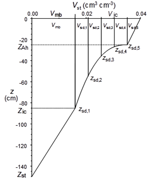
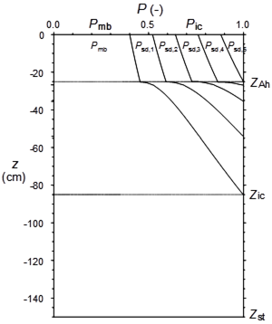
Shrinkage characteristics

The SWAP user needs to specify either the parameters of Kim’s or Hendriks’ relationship (see Section 6.2.2), or the values of typical points of the shrinkage characteristic curve. The different options and required parameters are listed in Table 6.1. The option to specify the original parameters of both relationships is especially relevant for the development of pedotransfer functions for shrinkage characteristics. The options to use typical points of the shrinkage characteristic curves are useful when limited information about the exact curves is available. When just a (rough) sketch of a curve is available it may be possible to recognize these typical points.

Table 6.1: Overview of required shrinkage parameters for clay and peat soils (Figure 6.5 and Figure 6.9).

Soil	SWSHRINP	SHRPARA	SHRPARB	SHRPARC	SHRPARD	SHRPARE
Rigid (0)	-	-	-	-	-	-
Clay (1)	1	α_K (e₀)	β_K	γ_K	-	-
	2	α_K (e₀)	ϑ_a	-	-	-
Peat (2)	1	e₀	ϑ_a	α_H	β_H	P_H
	2	e₀	ϑ_a	ϑ_r	ϑ_P	P_H
	3	e₀	ϑ_a	ϑ_i	e_i	-

For clay soils, the typical points are the void ratio e0 at \(\vartheta\) = 0 (\(\alpha_K\)) and the moisture ratio \(\vartheta_a\) at transition of normal to residual shrinkage (Figure 6.5). With these two input data, SWAP generates the parameters of Kim’s relationship. For peat soils, there are two options to use typical points of the shrinkage curve. The first, option 2 in Table 6.1, requires typical points with which the parameters of Hendriks’ curve can be generated. The second, option 3 in Table 6.1, enables to describe the shrinkage with three straight line-pieces.

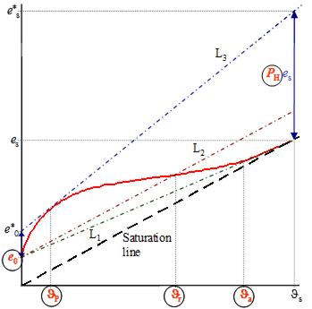
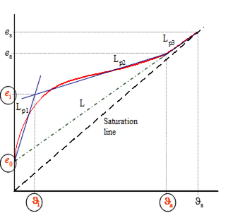
Option 2 requires the construction of three support-lines, L₁, L₂ and L₃, in the graph of the shrinkage curve (Figure 6.9). L₁ connects the points (0,\(e_0\)) and (\(\vartheta_s\), \(e_s\)). L₂ is parallel to the saturation line and starts at point (0,\(e_0\)). L₃ connects the points (0,\(e^*_0\)) and (\(\vartheta_s\), \(e^*_s\)) and is tangent to the shrinkage curve. In order to construct this line, parameter \(P_H\) should be found so that \(e^*_0\) = (1 + \(P_H\)) \(e_0\) and \(e^*_s\) = (1 + \(P_H\)) \(e_s\). This can easily be done by trial-and-error in a spreadsheet or on paper. When \(P_H\) < 0, L₂ must start at point (0,½\(e_0\)) instead of point (0,\(e_0\)) (e.g. samples A-15 and V-10 in Appendix J). For values of |\(P_H\)| < 0.1, option 3 is recommended (e.g. sample A-25 in Appendix J). Input parameters are (Table 6.1): \(e_0\), \(P_H\), \(\vartheta_a\) (moisture ratio at transition of ‘near-normal’ to ‘subnormal’ shrinkage on L₁, Figure 6.5), \(\vartheta_r\) (moisture ratio at intersection point of L₂ and curve) and \(\vartheta_P\) (moisture ratio at tangency point of L₃ to curve). Values must be given with an accuracy of at least 1% of saturated moisture ratio (\(\vartheta_s\)).

Option 3 requires the construction of three line-pieces L_p1, L_p2 and L_p3 and one support-line L in the graph of the shrinkage curve (Figure 6.9). L_p1 connects the points (0,\(e_0\)) and (\(\vartheta_i\),\(e_i\)), L_p2 the points (\(\vartheta_i\),\(e_i\)) and (\(\vartheta_a\),\(e_a\)), and L_p3 the points (\(\vartheta_a\),\(e_a\)) and (\(\vartheta_s\),\(e_s\)). L connects the points (0,\(e_0\)) and (\(\vartheta_s\),\(e_s\)). Point (\(\vartheta_a\),\(e_a\)) is situated on this line and represents the point of transition of ‘near-normal’ to ‘subnormal’ shrinkage. Point (\(\vartheta_i\),\(e_i\)) should be chosen in such a way that the three line-pieces describe the shrinkage curve as accurate as possible. For use in the model, L_p2 and L_p3 are much more important than L_p1. So emphasis should be put on these two line-pieces. Input parameters are (Table 6.1): \(e_0\), \(\vartheta_a\), \(e_i\) and \(\vartheta_i\).

If there is no information available to decide otherwise, thetcrmp could be taken at 90-100% \(\theta_{sat}\) (and may not exceed \(\theta_{sat}\)), geomfac as 3.0 and zncrar around -5.0 cm. The geometry factor may also be estimated as function of depth, with decreasing values for deeper soil layers as the overburden pressure of the soil on top may prevent the formation of structural cracks (Akker et al. 2013).

Measured shrinkage characteristics of seven clay profiles and four peat profiles in the Netherlands, as described respectively by Bronswijk and Evers-Vermeer (1990) and Hendriks (2004), are listed in Appendix J. Yule and Ritchie (1980a, 1980b) described shrinkage characteristics of eight Texas Vertisols, using small and large cores. Garnier et al. (1997) propose a simple evaporation experiment to determine simultaneously the moisture retention curve, hydraulic conductivity function and shrinkage characteristic.

Numerical stability

Numerical stability may at times cause problems in systems with macropore calculations. The following parameters are especially relevant in that respect:

swmbf: the type of flow considered is important, depending on the distribution between the main bypass and internal catchment domains. Switching between the types of flow may improve the simulation.
shapefacmp: this determines the exchange rate between macropores and matrix. Reducing this factor may improve stability, but will also lower the exchange fluxes.
numbit_crit: the default value of 3 may be too low for macropore simulations, as they generally require more iterations. It is advised to increase this value to 4 or 5.
dtmax: a too large maximum timestep may result in problems in case of sudden rainfall events. It is advised to use a maximum timestep of 0.01 d (15 minutes) to avoid numerical instabilities.

MACROPORE INPUT EXAMPLE

The typical macropore input parameters are discussed in this section. They are listed in Tip 6.2. The presented values concern a field experiment on water, bromide tracer and pesticide transport in a tile-drained field on clay soil (Scorza Júnior et al. 2004). The field was located in the riverine area in the central part of the Netherlands. The soil concerned light to moderate clay (30-55 mass-% clay) and the crop was winter wheat. At 320 cm depth the clay soil was underlain by a coarse sand aquifer.

Tip 6.2: SWAP input section for preferential flow due to macropores (*.swp; case Andelst).

**********************************************************************************
* Part 7: Preferential flow due to macropores

* Switch for macropore flow [0..1, I]:
  SWMACRO = 1                ! 0 = No macropore flow
                             ! 1 = Macropore flow

* If SWMACRO=1, specify:
* Switch for type of main bypass flow:
  SWMBF = 1                  ! 1 = Instantaneous bypass
                             ! 2 = Kinematic wave

* If kinematic wave (SWMBF=2), specify:
  NKWT = 2.0                 ! Kinematic exponent [2.0 .. 4.0 -, R]

* Switch for type of absorption [1..2, I]:
  SWABS = 1                  ! 1 = Sorptivity
                             ! 2 = Diffusion

* Switch for type of seepage [1..2, I]:
  SWSEP = 1                  ! 1 = Ernst
                             ! 2 = Youngs

* If SWMACRO = 1, specify macropore geometry variables:
  Z_ST = -220.0              ! Depth bottom static macropores [-1000..0 cm, R]
  Z_IC = -100.0               ! Depth bottom internal catchment domain [-1000..0 cm, R]
  VLMPSTSS = 0.04            ! Volume fraction of static macropores at soil surface [0..0.5 cm3/cm3, R]
  NUMSBDM = 4                ! Number of subdomains in internal catchment domain [0..20 -, I]
  DIPOMI = 10.0              ! Minimal diameter soil polygons (shallow) [0.1..1000 cm, R]
  DIPOMA = 50.0              ! Maximal diameter soil polygons (deep) [0.1..1000 cm, R]
  ZDIPOMA = -220.0           ! Depth below which soil polygons reach their maximum diameter  [-1000..0 cm, R]
                             ! (only required and used if VLMPSTSS = 0.0 and PPICSS = 0.0)
  ZNCRAR = -5.0              ! Depth at which dynamic crack area of soil surface is calculated 
                             ! (only used if soil above depth ZNCRAR is not rigid) [-100..0 cm, R]

* Optional macropore geometry variables:
  Z_TP = 0.0                 ! Depth top macropores for cover layer (default = 0.0) [-1000..0 cm, R]
  Z_MB50 = -160.0            ! Depth at which the static main bypass domain volume is half that at the top (default = (Z_IC+Z_ST)/2) [-1000..0 cm, R]
  
* If SWMACRO = 1 and NUMSBDM > 0, specifiy internal catchment geometry variables:
  PPICSS = 0.5               ! Proportion of internal catchment domain at soil surface [0..0.99 -, R]
 
* Optional internal catchment geometry variables:
  Z_AH = -26.0               ! Depth bottom A-horizon (default = bottom first node) [-1000..0 cm, R]
  RZAH = 0.0                 ! Fraction macropores ended at bottom A-horizon (optional; default 0.0) [0..1 -, R]
  POWM = 1.0                 ! Power M for freq. distr. curve internal catchment domain (optional; default 1.0) [0..100 -, R]
  SPOINT = 1.0               ! Symmetry point for freq. distr. curve (optional; default 1.0) [0..1 -, R]
  SWPOWM = 0                 ! Switch for double convex/concave freq. distr. curve (optional, Y=1, N=0; default: 0) [0..1 -, I]
  
* If SWMACRO = 1, specify macropore hydrological variables:
  PNDMXMP = 0.0              ! Threshold value for ponding on soil surface before overland flow into macropores starts [0..10 cm, R]
  SHAPEFACMP = 1.5           ! Shape factor for description of macropore water exchange with matrix (theoretically between 1 and 2) [0..100 -, R]
  CRITUNDSATVOL = 0.1        ! Critical value for undersaturation volume [0..10 cm, R]
  
* Switch for eliminating Darcy flow unsaturated zone (absorption):
  SWDARCY = 0                ! 0 = Eliminate Darcy flow
                             ! 1 = Do not eliminate Darcy flow 

* Switch for rapid drainage to drainage system (at least one drainage level needs to be specified) [0..1 -, I]:
  SWDRRAP = 1                ! 0 = no rapid drainage
                             ! 1 = rapid drainage

* If SWDRRAP = 1, specify rapid drainage parameters:
 RAPDRARESREF = 14.0         ! Reference rapid drainage resistance [0..1.E+10 /d, R] 
 RAPDRAREAEXP = 1.0          ! Exponent for reaction rapid drainage to dynamic crack width [0..100 -, R]
 NUMLEVRAPDRA = 1            ! Number of drainage system connected to rapid drainage [1..5, -, I] 

* If SWMACRO = 1, specify shrinkage characteristics:
* SWSOILSHR = Switch for kind of soil for determining shrinkage curve: 0 = rigid soil, 1 = clay, 2 peat [0..2 -, I]
* SWSHRINP  = Switch for determining shrinkage curve [1..2 -, I]:
*         1 = parameters for curve are given;
*         2 = typical points of curve are given 
* GEOMFAC   = Geometry factor (3.0 = isotropic shrinkage), [0..100, R]
*
* ShrParA to ShrParE = parameters for describing shrinkage curves, 
* depending on combination of SWSOILSHR and SWSHRINP [-1000..1000, R]:
* SWSOILSHR = 0               : 0 variables required (all dummies)
* SWSOILSHR = 1 and SWSHRINP 1: 3 variables required (ShrParA to ShrParC) (rest dummies)
* SWSOILSHR = 1 and SWSHRINP 2: 2 variables required (ShrParA to ShrParB) (rest dummies)
* SWSOILSHR = 2 and SWSHRINP 1: 5 variables required (ShrParA to ShrParE)
* SWSOILSHR = 2 and SWSHRINP 2: 5 variables required (ShrParA to ShrParE)
* SWSOILSHR = 2 and SWSHRINP 3: 4 variables required (ShrParA to ShrParD) (rest dummies)
SWSoilShr  SwShrInp  ThetCrMP  GeomFac ShrParA ShrParB ShrParC ShrParD ShrParE
        1          2        0.385      3.0   0.343  0.5390   0.0      0.0     0.0
        1          2        0.385      3.0   0.343  0.5392   0.0      0.0     0.0
        1          2        0.354      3.0   0.415  0.6350   0.0      0.0     0.0
        1          2        0.375      3.0   0.400  0.6400   0.0      0.0     0.0 
        1          2        0.422      3.0   0.412  0.7840   0.0      0.0     0.0 
        1          2        0.420      3.0   0.406  0.6883   0.0      0.0     0.0 
        1          2        0.499      3.0   0.495  0.9000   0.0      0.0     0.0 
* End of table

* If SWMACRO = 1, specify sorptivity characteristics:
* SWSORP      = Switch for kind of sorptivity function [1..2 -, I]:  
*           1 = Calculated from hydraulic functions according to Parlange (requires SORPFACPARL, rest dummies)
*           2 = Emperical function from measurements (requires SORPMAX, SORPALFA, rest dummies)
* SORPFACPARL = Factor for modifying Parlange function (optional; default 1.0) [0..100 -, R]
* SORPMAX     = Maximal sorptivity at theta residual [0..100 cm/d**0.5, R]
* SORPALFA    = Fitting parameter for emperical sorptivity curve [-10..10 -, R]
  SwSorp   SorpFacParl  SorpMax  SorpAlfa
        1         0.33       0.0       0.0
        1         0.33       0.0       0.0
        1         0.50       0.0       0.0
        1         0.50       0.0       0.0
        1         0.50       0.0       0.0
        1         0.50       0.0       0.0
        1         0.50       0.0       0.0
* End of table
**********************************************************************************

Akker, J. J. H. van den, R. F. A. Hendriks, J. Y. Frissel, K. Oostindie, and J. G. Wesseling. 2013. Gedrag van Verdroogde Kades; Fase b, c, d: Ontstaan En Gevaar van Krimpscheuren in Klei- En Veenkades. Alterra-Rapport 2473. Book. Alterra, Wageningen. https://edepot.wur.nl/297906.

Berg, F. van den, R. F. A. Hendriks, J. J. T. I. Boesten, et al. 2022. Revised Greenhouse Scenarios for Exposure of Aquatic Organisms to Plant Protection Products. WENR Rapport 3151. Book. Wageningen Environmental Research. https://doi.org/10.18174/564926.

Beven, K., and P. Germann. 1982. “Macropores and Water Flow in Soils.” Journal Article. Water Resources Research 18 (5): 1311–25. https://doi.org/10.1029/WR018i005p01311.

Booltink, H. W. G. 1993. Morphometric Methods for Simulation of Water Flow. PhD-Thesis. Book. Wageningen University, The Netherlands.

Bouma, J., and J. L. Anderson. 1973. “Relationships Between Soil Structure Characteristics and Hydraulic Conductivity.” Book Section to Field Soil Moisture Regime. SSSA Special Publ. No. 5., edited by R. R. Bruce. America Society of Agronomy, Madison, Wisconsin.

Bronswijk, J. J. B. 1988. “Modeling of Water Balance, Cracking and Subsidence of Clay Soils.” Journal Article. Journal of Hydrology 97 (3-4): 199–212. https://doi.org/10.1016/0022-1694(88)90115-1.

Bronswijk, J. J. B., and J. J. Evers-Vermeer. 1990. “Shrinkage of Dutch Clay Soil Aggregates.” Journal Article. Netherlands Journal of Agricultural Science 38 (2): 175–94. https://doi.org/10.18174/njas.v38i2.16603.

Bronswijk, J. J. B., W. Hamminga, and K. Oostindie. 1995. “Field-Scale Solute Transport in a Heavy Clay Soil.” Journal Article. Water Resources Research 31 (3): 517–26. https://doi.org/10.1029/94wr02534.

Dekker, L. W., and C. J. Ritsema. 1996. “Preferential Flow Paths in a Water Repellent Clay Soil with Grass Cover.” Journal Article. Water Resources Research 32 (5): 1239–49. https://doi.org/10.1029/96wr00267.

Ernst, L. F. 1956. “Calculation of the Steady Flow of Groundwater in Vertical Cross-Sections.” Journal Article. Netherlands Journal of Agricultural Science 4: 126–31. https://doi.org/10.18174/njas.v4i1.17793.

Ernst, L. F. 1962. Groundwater Flow in the Saturated Zone and Its Calculation When Parallel Open Conduits Are Present. PhD Thesis. Book. University of Utrecht, The Netherlands.

Garnier, P., M. Rieu, P. Boivin, M. Vauclin, and P. Baveye. 1997. “Determining the Hydraulic Properties of a Swelling Soil from a Transient Evaporation Experiment.” Journal Article. Soil Science Society of America Journal 61 (6): 1555–63. https://doi.org/10.2136/sssaj1997.03615995006100060003x.

Gerke, H. H., and M. T. van Genuchten. 1993. “Evaluation of a First-Order Water Transfer Term for Variably Saturated Dual-Porosity Flow Models.” Journal Article. Water Resources Research 29: 1225–38. https://doi.org/10.1029/92WR02467Digital.

Gerke, H. H., and M. T. van Genuchten. 1996. “Macroscopic Representation of Structural Geometry for Simulating Water and Solute Movement in Dual-Porosity Media.” Journal Article. Advances in Water Resources 19. https://doi.org/10.1016/0309-1708(96)00012-7.

Germann, P. F. 1985. “Kinematic Wave Approach to Infiltration and Drainage into and from Soil Macropores.” Journal Article. Transactions of the ASAE 28: 745–49. https://doi.org/10.13031/2013.32331.

Greco, R., R. F. A. Hendriks, and W. Hamminga. 1997. “Clay Soil Aggregate Sorptivity Measurements Under Different Water Contents.” Book Section to Proceedings of the National Hydraulics Conference, November 1996. Turin, Italy.

Hendriks, R. F. A. 2004. “An Analytical Equation for Describing the Shrinkage Characteristics of Peat Soils.” Book Section to Wise Use of Peatlands. Proceedings of the 12th International Peat Congress, edited by J. Päivänen. Tampere, Finland.

Hendriks, R. F. A., K. Oostindie, and P. Hamminga. 1999. “Simulation of Bromide Tracer and Nitrogen Transport in a Cracked Clay Soil with the FLOCR/ANIMO Model Combination.” Journal Article. Journal of Hydrology 215 (1-4): 94–115. https://doi.org/10.1016/S0022-1694(98)00264-9.

Hoogmoed, W. B., and J. Bouma. 1980. “A Simulation Model for Predicting Infiltration into a Cracked Clay Soil.” Journal Article. Soil Science Society of America Journal 44: 458–61. https://doi.org/10.2136/sssaj1980.03615995004400030003x.

Kim, D. J. 1992. Characterization of Swelling and Shrinkage Behaviour, Hydraulic Properties and Modelling of Water Movement in a Physically Ripening Marine Clay Soil. PhD Thesis. Book. Catholic University Leuven, Belgium.

Larsbo, M., and N. Jarvis. 2003. MACRO 5.0. A Model of Water Flow and Solute Transport in Macroporous Soil. Technical Decripition. Book. Swedish University of Agricultural Sciences.

Nieber, J. L., T. S. Steenhuis, T. Walter, and M. Bakker. 2006. “Enhancement of Seepage and Lateral Preferential Flow by Biopores on Hillslopes.” Journal Article. Biologia 61: S225–28. https://doi.org/10.2478/s11756-006-0162-1.

Parlange, J. Y. 1975. “On Solving the Flow Equation in Unsaturated Soils by Optimization: Horizontal Infiltration.” Journal Article. Soil Science Society of America Proceedings 39: 415–18. https://doi.org/10.2136/sssaj1975.03615995003900030019x.

Peters, A., W. Durner, and G. Wessolek. 2011. “Consistent Parameter Constraints for Soil Hydraulic Functions.” Journal Article. Advances in Water Resources 34: 1352–65. https://doi.org/10.1016/j.advwatres.2011.07.006.

Philip, J. R. 1957. “The Theory of Infiltration: 4. Sorptivity and Algebraic Infiltration Equations.” Journal Article. Soil Science 84: 257–65.

Rijniersce, K. 1983. A Simulation Model for Physical Ripening in the IJsselmeerpolders. Book. Rijksdienst voor IJsselmeerpolders. Lelystad, The Netherlands.

Scorza Júnior, R. P., J. H. Smelt, J. T. I. Boesten, R. F. A. Hendriks, and S. E. A. T. M. van der Zee. 2004. “Preferential Flow of Bromide, Bentazon and Imidacloprid in a Dutch Clay Soil.” Journal Article. Journal of Environmental Quality 33: 1473–86. https://doi.org/10.2134/jeq2004.1473.

Sidle, R. C., S. Noguchi, Y. Tsuboyama, and K. Laursen. 2001. “A Conceptual Model of Preferential Flow Systems in Forested Hillslopes: Evidence of Self-Organization.” Journal Article. Hydrological Processes 15 (10): 1675–92. https://doi.org/10.1002/hyp.233.

Stroosnijder, L. 1975. Infiltration and Redistribution of Water in the Soil. PhD Thesis. Book. Wageningen University, Wageningen, The Netherlands.

Thoma, S. G., D. P. Gallegos, and D. M. Smith. 1992. “Impact of Fracture Coatings on Fracture/Matrix Flow Interactions in Unsaturated Porous Media.” Journal Article. Water Resources Research 28 (5): 1357–67. https://doi.org/10.1029/92wr00167.

Van Dam, J. C., and R. A. Feddes. 2000. “Numerical Simulation of Infiltration, Evaporation and Shallow Groundwater Levels with the Richards Equation.” Journal Article. Journal of Hydrology 233: 72–85. https://doi.org/10.1016/S0022-1694(00)00227-4.

Van Genuchten, M. Th. 1980. “A Closed Form Equation for Predicting the Hydraulic Conductivity of Unsaturated Soils.” Journal Article. Soil Science Society of America Journal 44: 892–98. https://doi.org/10.2136/sssaj1980.03615995004400050002x.

Youngs, E. G. 1980. “The Analysis of Groundwater Seepage in Heterogeneous Aquifers.” Journal Article. Hydrological Sciences Journal 25 (2): 155–65. https://doi.org/10.1080/02626668009491920.

Yule, D. F., and J. T. Ritchie. 1980a. “Soil Shrinkage Relationships of Texas Vertisols: I. Small Cores.” Journal Article. Soil Science Society of America Journal 44: 1285–91. https://doi.org/10.2136/sssaj1980.03615995004400060031x.

Yule, D. F., and J. T. Ritchie. 1980b. “Soil Shrinkage Relationships of Texas Vertisols: II. Large Cores.” Journal Article. Soil Science Society of America Journal 44: 1291–95. https://doi.org/10.2136/sssaj1980.03615995004400060032x.