| Scale of application | No of systems | Drainage flux relation | Drainage level |
|---|---|---|---|
| Field | Single drainage system | Hooghoudt or Ernst equation | Specified in model input |
| Tabulated input | Implicitly included in tabulated input | ||
| Regional | Single drainage system | Tabulated input | Implicitly included in tabulated input |
| Multiple drainage system | Drainage resistance per sub-system | Specified in model input per drainage system | |
| Drainage resistance per sub-system dependent on wetted perimeter of drains | Specified in model input per drainage system | ||
| Simulated (see Chapter 5) |
4 Surface runoff, interflow and drainage
The interaction between soil water and surface water is of importance in lowland areas. Dependent on the specific setting in the landscape of the field studied, different types of pathways and interconnections may play a role.
Surface runoff that occurs when the rainfall rate exceeds the infiltration rate is called Horton overland flow. A second form of runoff occurs after the water storage volume of a soil has been exceeded, which means that the groundwater table has reached the soil surface. This runoff is commonly called the Dunne overland flow. It occurs in areas with a shallow groundwater table and moderate rainfall of long duration.
Interflow can be defined as the near-surface flow of water within the soil profile resulting in seepage to a stream channel within the time frame of a storm hydrograph. Interflow involves both unsaturated and saturated flows, the latter being in zones of limited vertical extent caused by soil horizons impeding vertical percolation. The mechanisms by which subsurface flow enters streams quickly enough to contribute to streamflow responses to individual rainstorms are summarized in various publications (Beven 1989).
Infiltration excess moves slowly downwards and once it has reached the saturated zone, it is called ground water. Ground water moves downward and laterally through the subsurface and eventually discharges through tile drains, field ditches or other open conduits. A tile drain is a perforated conduit, such as tile, pipe or tubing, installed below the ground surface to intercept and convey drainage water.
The SWAP model can take account for the different types of interconnections between soil moisture/groundwater and surface water by offering options for describing surface runoff as a non-linear function of water storage on the field, interflow as a non-linear function of the groundwater elevation when it has reached the near-surface zone and the discharge to a series of drainage systems. Options to simulate dynamically the levels in surface water systems provide the possibility to describe the feedback and the close interconnection between groundwater and surface water in stream valleys and polders.
4.1 Surface runoff
Surface runoff is one of the terms in the water balance of the ponding reservoir. The ponding reservoir stores a certain amount of excess water on top of the soil surface (Figure 4.1).
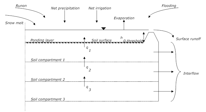
The water balance of the ponding reservoir is governed by:
\[ \frac{\Delta h_0}{\Delta t} = q_{\text{prec}} + q_{\text{irri}} + q_{\text{melt}} + q_{\text{runon}} + q_{\text{inun}} + q_1 - q_{\text{e,pond}} - q_{\text{runoff}} - q_{tl} \tag{4.1}\]
Where \(\Delta h_0\) is the storage change of the ponding reservoir (cm d-1), \(q_\text{prec}\) is the precipitation flux subtracted with interception (cm d-1), \(q_\text{irri}\) is the irrigation flux subtracted with interception (cm d-1), \(q_1\) is the flux from the first model compartment to the ponding layer (cm d-1), \(q_\text{melt}\) is snowmelt (cm d-1), \(q_\text{runon}\) is the runon flux of water which enters the field from an upstream adjacent field (cm d-1), \(q_\text{inun}\) is the inundation or flooding from surface water to the field (cm d-1), \(q_\text{runoff}\) is surface runoff flux (cm d-1) and \(q_\text{e,pond}\) is the evaporation flux of the open water stored on the soil surface (cm d-1) and \(q_{tl}\) is the runoff into the macropores (cm d-1, see Section 6.3.1).
Surface runoff occurs when the water storage in the ponding layer exceeds the critical depth of \(h_{0,\text{threshold}}\) (cm):
\[ q_{\text{runoff}} = \frac{1}{\gamma} \left( \max \left( 0, \left(h_0 - h_{0,\text{threshold}}\right) \right)^\beta \right) \tag{4.2}\]
where \(h_0\) is the ponding depth of water (cm) on the soil surface, \(\gamma\) is a resistance parameter (cm\(\beta\)-1 d) and \(\beta\) is an exponent (-) in the empirical relation. Inundation of the field from an adjacent water course can be simulated when the surface water level exceeds both \(h_0\) and \(h_{0,\text{threshold}}\). This option is only available when the so-called extended drainage option is chosen (see Chapter 5).
4.2 Interflow
In some applications, one may wish to describe an interflow system, which has a rapid discharge with short residence times of the water in the soil system. If the groundwater level \(\phi_\text{gwl}\) is higher than the hydraulic head of the drain \(\phi_\text{drain,n}\), the interflow flux is optionally calculated as:
\[ q_\text{drain,n} = \frac{\phi_\text{gwl} - \phi_\text{drain,n}}{\max \left( \gamma_\text{min}, 1 \cdot \phi_\text{gwl} - \gamma_\text{ref} \right)} \tag{4.3}\]
or as:
\[ q_\text{drain,n} = A_\text{interflow} \left(\phi_\text{gwl} - \phi_\text{drain,n}\right)^{B_\text{interflow}} \tag{4.4}\]
where \(q_\text{drain,n}\) is the interflow flux (cm d-1), \(\gamma_\text{min}\) and \(\gamma_\text{ref}\) are the minimum and the reference resistance related to the interflow process, ‘1’ is a factor that expresses the unit conversion and is equal to one (d cm-1) in this case. \(A_\text{interflow}\) is a conductance parameter (cm1-B d-1) and \(B_\text{interflow}\) is an exponent (-) in the empirical relation. The subscript \(n\) points to the rule that in the SWAP model interflow is always assigned to the highest order of distinguished drainage systems.
4.3 Drain discharge
Although the entity for which the SWAP model operates is at field scale, the model is used both for field studies and for regional studies. The different spatial scales of operation are expressed among other things by the type of drainage relation and its associated parameters chosen. For the purpose of a drainage system at field scale, one may use one of the classical drainage equations, but for simulation of water discharge in the spatial entity of a sub-catchment, the use of a multiple drainage system formulation is more convenient. Table 4.1 provides a brief overview of the drainage options available in the SWAP model. Additionally, options are available to take account for the influence of surface water management strategies on soil water flow and drain discharge. The background and the implementation of this option is presented in Chapter 5.
The options provided by the SWAP model are limited to lowland conditions. Subsurface groundwater flow and drainage response of sloping fields can better be described by 2D or 3D models or Boussinesq-equation based models. Another limitation of the drainage equations involves the steady-state assumption. Hysteresis phenomena in the groundwater – discharge relation as they can be observed in experimental data are attributed to the different possible shapes of the groundwater elevation surface pertaining to one groundwater level value. Although there are possibilities to conceptualize the 2D groundwater depth discharge relation for nonsteady-state conditions (Kraijenhoff van de Leur 1958; Wesseling and Wesseling 1984), this is not implemented. These relations consider only one over-all value for the storage coefficient and neglect the influence of the pressure head variations in space and time on the storativity. If such phenomena are of interest for drainage flow simulations, the reader is referred to 2D and 3D models as MODFLOW-VSF (Thoms, Johnson, and Healy 2006), SUTRA (Voss and Provost 2002), FEMWATER (Lin et al. 1997), and HYDRUS (Šimůnek, Šejna, and Genuchten 2007).
The drainage flux are incorporated in the numerical solution to the Richards equation (see Chapter 2) by specifying it as a sink term. The drainage relations presented in Section 4.3 are conceptualizations of 2D and 3D saturated groundwater flow to surface water systems and are based on the head difference between groundwater elevation and drainage level. Assignment of drainage sink term values in the Richards equation involves a conceptualization of the 2D and 3D flow field, which is briefly explained in Section 4.4. Optionally, to provide possibilities to compare the SWAP model with other 1D soil moisture models as HYDRUS1D (Šimůnek et al. 1998), the drain flux can be described as a vertical flow in the model, which leaves the flow domain at the bottom.
It should be noticed that the calculation of drainage resistance should be attuned to the definition of the groundwater elevation as one of the driving forces of groundwater discharge and to the lower boundary condition one wants to impose. The general formulation of the drainage equation:
\[ q_\text{drain} = \frac{\left(\phi_\text{gwl} \, \text{or} \, \phi_\text{avg}\right) - \phi_\text{drain}}{\gamma_\text{drain}} \tag{4.5}\]
where \(\phi_{\text{gwl}}\) is the phreatic groundwater level midway between the drains or ditches (cm), \(\phi_\text{avg}\) is the averaged phreatic groundwater level midway between the drains or ditches (cm), \(\phi_\text{drain}\) is the drainage level (cm) and \(\gamma_\text{drain}\) is the drainage resistance (d).
Drainage relations are generally derived from the groundwater elevation as a function of distance. An example is given in Figure 4.2.
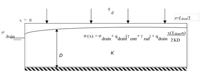
For drainage design purposes, one may be interested in the maximum groundwater elevation (\(\phi_\text{gw}\)), but for the analysis of regional water management, the average groundwater elevation (\(\phi_\text{avg}\)) is often a key variable to be studied. The different backgrounds reveal themselves in the manner the drainage flux is calculated. For field applications, the relation between the drainage flux and the groundwater elevation can be expressed by the Ernst equation, modified with respect to the introduction of an additional entrance resistance:
\[ \phi_\text{gwl} = \phi_\text{drain} + q_\text{drain} \left(\gamma_\text{entr} + \gamma_\text{rad} + \frac{L_\text{drain}^2}{8KD}\right) \rightarrow q_\text{drain} = \frac{\phi_\text{gwl} - \phi_\text{drain}}{\gamma_\text{entr} + \gamma_\text{rad} + \frac{L_\text{drain}^2}{8KD}} \tag{4.6}\]
and for regional applications:
\[ \phi_\text{avg} = \phi_\text{drain} + q_\text{drain} \left(\gamma_\text{entr} + \gamma_\text{rad} + \frac{L_\text{drain}^2}{12KD}\right) \rightarrow q_\text{drain} = \frac{\phi_\text{avg} - \phi_\text{drain}}{\gamma_\text{entr} + \gamma_\text{rad} + \frac{L_\text{drain}^2}{12KD}} \tag{4.7}\]
By comparing Equation 4.6 with Equation 4.7 it can be seen that the two definitions of \(\gamma_{\text{drain}}\) in the equations differ by the so-called shape factor. The shape factor \(\alpha\) is the ratio between the mean and the maximum groundwater level elevation above the drainage base:
\[ \alpha = \frac{\phi_\text{avg} - \phi_\text{drain}}{\phi_\text{gwl} - \phi_\text{drain}} \tag{4.8}\]
The shape factor depends on the vertical, horizontal, radial, and entrance resistances of the drainage system (Ernst 1978a, 1978b). For regional situations, where the ‘horizontal’ resistance to flow plays an important role, the shape factor is relatively small (approximately 0.7). The smaller the horizontal resistance becomes, the more ‘rectangular’ shaped the water table: in the most extreme case with all the resistance concentrated in the direct vicinity of the channel, the water table is level, except for the abrupt decrease towards the drainage base. In that case, the shape factor approaches unity.
It should be noted that the parameters chosen to describe the relation between discharge and groundwater elevation should be attuned to the hydrological schematization. The combination of a Cauchy condition for the bottom boundary with a drainage relation for the lateral boundary may require another formula (De Lange 1999) than the one usually applied for drainage combined with a flux bottom boundary condition. Also, the coupling of the SWAP model to a regional groundwater model by exchanging information concerning fluxes and hydraulic heads at the bottom of the schematization may require alternative formulations for the drainage equation to be used.
The influence of frost at a certain depth can optionally be accounted for by the reduction of prevailing drainage fluxes at that depth similar to the reduction of hydraulic conductivities (see Chapter 2).
4.3.1 Field scale drainage relation according to Hooghoudt and Ernst
The drainage equations of Hooghoudt and Ernst allow the evaluation of drainage design and are based on the drainage flux as a function of the head difference the maximum groundwater elevation midway between the drains and the drainage level. Depending on the position of the groundwater level, the drainage level, and the possibility for water supply in the surface water system, the channels will act as either drainage or sub-irrigation media. The theory behind the field drainage equations used for drainage design purposes is summarized by Ritzema (1994). Five typical drainage situations are distinguished (Table 4.2). For each of these situations, the drainage resistance \(\gamma_\text{drain}\) (d) can be defined.
| Case | Schematization | Soil profile | Drain position |
|---|---|---|---|
| 1 | 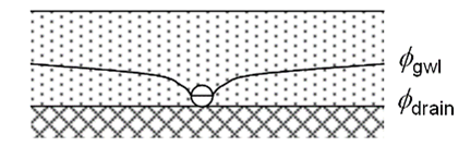 |
Homogeneous | On top of impervious layer |
| 2 | 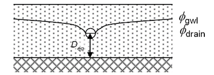 |
Homogeneous | Above impervious layer |
| 3 | 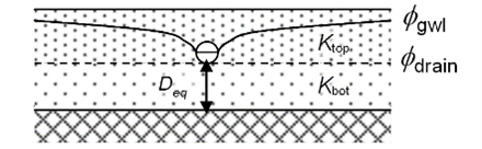 |
Two layers | At interface of two soil layers |
| 4 | 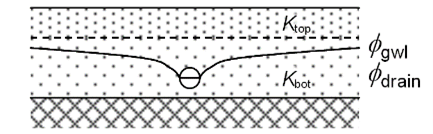 |
Two layers (Ktop << Kbot) | In bottom layer |
| 5 | 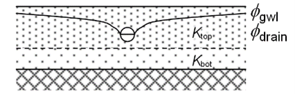 |
Two layers (Ktop >> Kbot) | In top layer |
Case 1: Homogeneous profile, drain on top of impervious layer
The drainage resistance is calculated as:
\[ \gamma_\text{drain} = \frac{L_\text{drain}^2}{4K_\text{hprof} \left(\phi_\text{gwl} - \phi_\text{drain}\right)} + \gamma_\text{entr} \tag{4.9}\]
with \(K_\text{hprof}\) the horizontal saturated hydraulic conductivity above the drainage basis (cm d-1), \(L_\text{drain}\) the drain spacing (cm), and \(\gamma_\text{entr}\) the entrance resistance into the drains and/or ditches (d). The value for \(\gamma_\text{entr}\) can be obtained, analogous to the resistance value of an aquitard, by dividing the ‘thickness’ of the channel walls with the permeability. If this permeability does not differ substantially from the conductivity in the surrounding subsoil, the numerical value of the entry resistance will become relatively minor.
Case 2: Homogeneous profile, drain above impervious layer
This drainage situation has been originally described by Hooghoudt (1940). An extension for the entrance resistance has been added later on. The drainage resistance follows from:
\[ \gamma_\text{drain} = \frac{L_{\text{drain}}^2}{8K_\text{hprof} D_\text{eq} + 4K_\text{hprof} (\phi_\text{gwl} - \phi_\text{drain})} + \gamma_\text{entr} \tag{4.10}\]
where \(D_{\text{eq}}\) is the equivalent depth (cm) that accounts for the extra head loss near the drains caused by converging flow lines (Hooghoudt 1940). The numerical solution of Van der Molen and Wesseling (1991) is employed to obtain an estimate for \(D_{\text{eq}}\). A characteristic dimensionless length scale \(x\) is used:
\[ x = 2\pi \frac{\left(\phi_{\text{drain}} - z_\text{imp}\right)}{L_\text{drain}} \tag{4.11}\]
where \(z_{\text{imp}}\) is the level of the impervious layer. The equivalent depth \(D_{\text{eq}}\) is approximated for three ranges of \(x\) as:
If \(x < 10^{-6}\): \[ D_\text{eq} = \phi_\text{drain} - z_\text{imp} \tag{4.12}\]
If \(10^{-6} < x < 0.5\): \[ D_\text{eq} = \frac{L_\text{drain}}{\frac{8}{\pi} \ln\left(\frac{\phi_\text{drain} - z_\text{imp}}{\pi r_\text{drain}}\right) + \frac{L_\text{drain}}{\phi_\text{drain} - z_\text{imp}}} \tag{4.13}\]
If \(x > 0.5\): \[ D_\text{eq} = \frac{L_\text{drain}}{\frac{8}{\pi} \left(\ln\left(\frac{L_\text{drain}}{\pi r_\text{drain}}\right) + \sum_{k=1,3,5,\dots}^\infty \frac{4e^{-2kx}}{k(1-e^{-2kx})}\right)} \tag{4.14}\]
Case 3: Heterogeneous soil profile, drain at interface between both soil layers
The drainage resistance follows from:
\[ \gamma_\text{drain} = \frac{L_\text{drain}^2}{8K_\text{hbot} D_\text{eq} + 4K_\text{htop} (\phi_\text{gwl} - \phi_\text{drain})} + \gamma_\text{entr} \tag{4.15}\]
with \(K_\text{htop}\) and \(K_\text{hbot}\) the horizontal saturated hydraulic conductivity (cm d-1) of upper and lower soil layer, respectively. The equivalent depth \(D_\text{eq}\) is calculated using Equation 4.11 to Equation 4.14.
Case 4: Heterogeneous soil profile, drain in bottom layer
The drainage resistance is calculated according to Ernst (1956) with later extensions for the entrance resistance as:
\[ \gamma_\text{drain} = \gamma_\text{ver} + \gamma_\text{hor} + \gamma_\text{rad} + \gamma_\text{entr} \tag{4.16}\]
where \(\gamma_\text{ver}\), \(\gamma_\text{hor}\), \(\gamma_\text{rad}\) and \(\gamma_\text{entr}\) are the vertical, horizontal, radial, and entrance resistance (d-1), respectively. The vertical resistance is calculated by:
\[ \gamma_\text{ver} = \frac{\phi_\text{gwl} - z_\text{int}}{K_\text{vtop} z_\text{drain\_int}/K_\text{vbot}} \tag{4.17}\]
with \(z_{\text{int}}\) the level of the transition (cm) between the upper and lower soil layer, and \(K_{\text{vtop}}\) and \(K_{\text{vbot}}\) the vertical saturated hydraulic conductivity (cm d\(^{-1}\)) of the upper and lower soil layer, respectively. The horizontal resistance is calculated as:
\[ \gamma_{\text{hor}} = \frac{L_{\text{drain}}^2}{8K_{\text{hbot}} D_{\text{bot}}} \tag{4.18}\]
with \(D_{\text{bot}}\) the depth of the contributing layer below the drain level (cm), which is calculated as the minimum of \((\phi_{\text{drain}} - z_{\text{imp}})\) and \(\frac{1}{4} L_{\text{drain}}\). The radial resistance is calculated using:
\[ \gamma_\text{rad} = \frac{L_\text{drain}}{\pi\sqrt{K_\text{hbot} K_\text{vbot}}} \ln\left(\frac{D_\text{bot}}{u_\text{drain}}\right) \tag{4.19}\]
with \(u_\text{drain}\) the wet perimeter (cm) of the drain.
Case 5: Heterogeneous soil profile, drain in top layer
Again, the approach of Ernst (1956), with later extensions for the entrance resistance, is applied. The resistances are calculated as:
\[ \gamma_\text{ver} = \frac{\phi_\text{gwl} - \phi_\text{drain}}{K_\text{vtop}} \tag{4.20}\]
\[ \gamma_\text{hor} = \frac{L_\text{drain}^2}{8K_\text{htop} D_\text{top} + 8K_\text{hbot} D_\text{bot}} \tag{4.21}\]
\[ \gamma_\text{rad} = \frac{L_\text{drain}}{\pi \sqrt{K_\text{hbot} K_\text{vbot}}} \ln\left(\frac{g_\text{drain} \left(\phi_\text{drain} - z_\text{int}\right)}{u_\text{drain}}\right) \tag{4.22}\]
with \(D_\text{top}\) equal to \((\phi_\text{drain} - z_\text{int})\) and \(g_\text{drain}\) is the drain geometry factor, to be specified in the input. The value of \(g_\text{drain}\) in Equation 4.22 depends on the ratio of the hydraulic conductivity of the bottom (\(K_\text{hbot}\)) and the top (\(K_\text{htop}\)) layer. Ernst (1962) distinguished the following situations:
If \(K_\text{hbot} / K_\text{htop} < 0.1\): the bottom layer can be considered impervious, and the case is reduced to a homogeneous soil profile with \(g_\text{drain} = 1\).
If \(0.1 < K_\text{hbot} / K_\text{htop} < 50\): \(g_\text{drain}\) depends on the ratios \(K_\text{hbot} / K_\text{htop}\) and \(D_\text{bot} / D_\text{top}\), as given in Table 4.3.
If \(K_{\text{hbot}} / K_{\text{htop}} > 50\): \(g_{\text{drain}} = 4\).
| 1 | 2 | 4 | 8 | 16 | 32 | |
|---|---|---|---|---|---|---|
| 1 | 2.0 | 3.0 | 5.0 | 9.0 | 15.0 | 30.0 |
| 2 | 2.4 | 3.2 | 4.6 | 6.2 | 8.0 | 10.0 |
| 3 | 2.6 | 3.3 | 4.5 | 5.5 | 6.8 | 8.0 |
| 5 | 2.8 | 3.5 | 4.4 | 4.8 | 5.6 | 6.2 |
| 10 | 3.2 | 3.6 | 4.2 | 4.5 | 4.8 | 5.0 |
| 20 | 3.6 | 3.7 | 4.0 | 4.2 | 4.4 | 4.6 |
| 50 | 3.8 | 4.0 | 4.0 | 4.0 | 4.2 | 4.6 |
4.3.2 Field scale drainage relation defined by a tabulated function
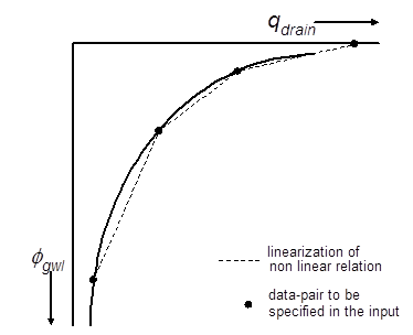
The SWAP model provides an option to specify a tabulated drainage flux relationship as a function of the groundwater level (\(\phi_\text{gwl}\)). When this option is chosen, one should specify a number of \((\phi_\text{gwl}, q_\text{drain})\) data-pairs. For a linear relation, only two data-pairs suffice, but a non-linear relation requires more data-pairs. A non-linear relation can result from:
- describing the drainage flux by the Hooghoudt equation;
- an analysis of the flux relation in a stratified profile by means of a numerical model;
- an analysis of measured field data.
The general shape of such a relation is illustrated in Figure 4.3. Specifying a non-linear relation by means of a tabulated function involves a linearization since flux values are derived by linear interpolation. Specifying more data pairs can reduce the inaccuracy resulting from this type of linearization.
4.3.3 General aspects of regional scale drainage
The groundwater-surface water system is described at the scale of a horizontal sub-region. A network of drainage devices consists of a hierarchical system of different order and incision depth, but only a single representative groundwater level is simulated for a sub-region, which is ‘stretched’ over a scale that in reality involves a variety of groundwater levels. In the following, due consideration will be given to the schematization of the surface water system, the simulation of drainage/sub-irrigation fluxes, and the handling of an open surface water level.
The regional surface water system consists of a hierarchical system of different order drainage devices (Figure 4.4), each with its own with bed level, bed width, side-slope, and spacing conveyance capacity. The drainage devices can be connected to each other in different ways. In the man-made the ditches of the network systems act as perennial streams, connected to larger canals with a nearly equal surface water level. In the alluvial sandy areas of the Netherlands, the smaller streams may have intermittent character which only discharge water in periods with rainwater excess.
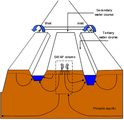
It should be noted that, contrary to the classification notation used in geo-morphological sciences, in this report the stream and canal order is dictated by the level of the stream bed or water level (drainage level) compared to the land surface level: the deeper the drainage level, the lower the classification index.
The representative distance between drain devices \(L_\text{drain,i}\) (m) is derived by dividing the area of the subregion \(A_\text{reg}\) (m2) by the total length of the ith order channels, \(l_\text{drain,i}\) (m):
\[ L_\text{drain,i} = \frac{A_\text{reg}}{l_\text{drain,i}} \tag{4.23}\]
In the surface water model, we assume that the different channels orders are connected in a dendritic manner. Together they form a surface water ‘control unit’ with a single outlet (indicated by the weir in Figure 4.4) and, if present, a single inlet. The surface water level at the outlet is assumed to be omnipresent in the subregion. Friction losses are neglected, and thus the slope of the surface water level is assumed to be zero. This means that in all parts of the subregion the surface water level has the same depth below the soil surface.
In the so-called ‘multi-level’ drainage or sub-irrigation approach employed by the SWAP model, it is possible that more than one type of surface water channel becomes active simultaneously. In the following, we will refer to channels in terms of their ‘order’ if their role as part of the surface water system is being considered. When considering their drainage characteristics, we will refer to them in terms of their ‘level’.
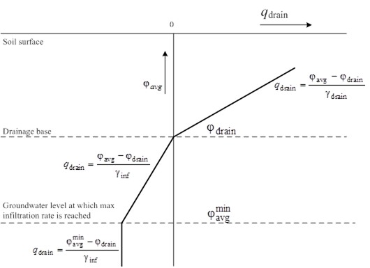
The SWAP model has the option for specifying resistances for calculating the sub-irrigation flux that differ from the resistance values used for drainage. An additional model option involves the limitation of the sub-irrigation rate by defining the groundwater level \(\phi_\text{avg}^\text{min}\) at which the maximum sub-irrigation rate is reached. Such a limitation is needed because the sub-irrigation rate does not increase infinitely when the groundwater level lowers.
4.3.4 Regional scale drainage relation defined by a tabulated function
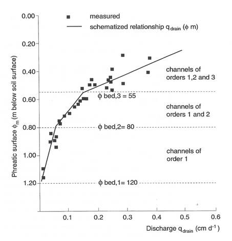
An example of a non-linear relation between discharge and groundwater elevation resulting from an analysis of observed field data is presented in Figure 4.6. It can be seen from this figure that the non-linear relation may be linearized to a piece-wise linear relation in which each part of this relation corresponds to a cer¬tain type of drainage system. From Figure 4.6 one can infer that the drainage base of the larger channels is roughly at \(z\) = -120 cm, as no discharges were measured below that level. The schematized \(q_\text{drain} (\phi_\text{avg})\)-relationship has transition points at mean groundwater levels of 80 and 55 cm below soil surface. These transition points correspond to the ‘representative’ bed levels of the second and third order channels. These levels could be imposed to the SWAP model as drainage levels.
4.3.5 Multi-level drainage with fixed resistances and imposed drainage levels
In the context of multi-level drainage with fixed resistances and imposed drainage levels, before any calculation of the drainage/sub-irrigation rate, it’s determined whether the flow situation involves drainage, sub-irrigation, or neither. No drainage or sub-irrigation will occur if both the groundwater level and surface water level are below the drainage base.
Drainage occurs only if:
- the groundwater level is higher than the channel bed level;
- the groundwater level is higher than the surface water level.
Sub-irrigation occurs only if:
- the surface water level is higher than the channel bed level;
- the surface water level is higher than the groundwater level.
In both cases, the drainage base, \(\phi_{\text{drain}}\) (cm), is taken as either the surface water level, \(\phi_{\text{sur}}\) (cm), or the channel bed level, \(z_{\text{bed}}\) (cm), whichever is higher:
\[ \phi_\text{drain} = \max\left(\phi_\text{sur}, z_\text{bed}\right) \tag{4.24}\]
The hydraulic head \(\phi\) is defined positive upward, with zero at the soil surface.
The drainage/infiltration flux \(q_\text{drain,i}\) (cm d-1) to/from each surface water system i is calculated from the linear relation:
\[ q_\text{drain,i} = \frac{\phi_\text{avg} - \phi_\text{drain,i}}{\gamma_\text{drain,i}} \tag{4.25}\]
where \(\phi_\text{drain,i}\) is the drainage base equal to the surface water level of system i (cm below the soil surface), and \(\gamma_\text{drain,i}\) is the drainage resistance of system i (d). Similar to the single-level drainage case, a drainage level is only ‘active’ if either the groundwater level or the surface water level is higher than the channel bed level. The drainage base is determined separately for each drainage level. In computing the total flux \(q_\text{drain}^\text{tot}\) to/from surface water, the contributions of the different channel orders are simply summed:
\[ q_\text{drain}^\text{tot} = \sum_{i=1}^{n} q_\text{drain,i} \tag{4.26}\]
4.3.6 Multi-level drainage with surface water dependent resistances and simulated drainage levels
In most applications, the control unit involves the primary watercourse; the largest canals with the deepest channels beds. An option is available to specify that the primary watercourse, e.g., a large river, functions separately from the other watercourses within the sub-regional surface water system. This implies that primary watercourses have their own surface water level, which should be specified in the input. In reality, there may be some interaction between the primary watercourse and the control unit, such as a pumping station for drainage water removal, and/or an inlet for external surface water supply (Figure 4.4). The hydraulics of such structures are not included in the model. Conveyance processes within the surface water devices are not described.
Contrary to the option described in Section 4.3.5, the influence of the surface water level on drainage resistances can be accounted for by distinguishing two parts of the resistance: 1) a part independent of the surface water level and 2) a part adjusted by the level. For the drainage case:
\[ \gamma_\text{drain,i} = \gamma_\text{drain,i}^{0} + \gamma_\text{entr,i}^{*} \frac{L_\text{drain,i}}{u_\text{drain,i}} \tag{4.27}\]
And for the sub-infiltration case:
\[ \gamma_\text{infil,i} = \gamma_\text{infil,i}^{0} + \gamma_\text{exit,i}^{*} \frac{L_\text{drain,i}}{u_\text{drain,i}} \tag{4.28}\]
where \(\gamma_\text{drain,i}^{0}\) and \(\gamma_\text{infil,i}^{0}\) are the level-independent parts of the drainage and infiltration resistance, respectively, and \(\gamma_\text{entr,i}^{*}\) and \(\gamma_\text{exit,i}^{*}\) are the entrance and exit resistance factor per unit drain distance (\(L_\text{drain,i}\)) and divided by the wetted perimeter (\(u_\text{drain,i}\)). The radial resistance has been lumped with the entrance or exit resistance. Assuming a trapezoidal cross-section of the watercourses, the wetted perimeter can be calculated as:
\[ u_\text{drain,i} = w_\text{bed,i} + \max\left(0,\ 2 \cdot \left(\phi_\text{sur} - z_\text{bed,i}\right) \sqrt{1 + \frac{1}{\alpha_\text{sl,i}^{2}}}\right) \tag{4.29}\]
where \(w_\text{bed,i}\) is the channel bed width (cm) and \(\alpha_\text{sl,i}\) (-) is the slope of the channel bank.
Another feature of this model option includes the ability to simulate the flooding of the field when the surface water level higher appears to be higher than both the ponding sill and the ponding level or groundwater level (Figure 4.7).

The model concept for flooding does not take account for the resistance of water flowing on the field surface and an immediate equilibrium between the ponding level and the surface water level is assumed when flooding occurs.
4.4 Distribution with depth of drainage fluxes
4.4.1 Implicit approach of travel times
In this section, the concept for the distribution of drainage fluxes with depth as one of the sink terms in the SWAP model is described. Although the concept discussed here is valid for a region having any number of drainage levels, only three drainage systems are considered for simplicity.
One-dimensional leaching models generally represent a vertical soil column. Within the unsaturated zone, solutes are transported by vertical water flows, whereas in the saturated zone, the drainage discharge can have a three-dimensional flow pattern. Van Ommen et al. (1989) showed that for a simple single-level drainage system, the travel time distribution is independent of the size and shape of the recharge area. Under these assumptions, the average concentration in drainage water can mathematically be described by the linear behavior of a single reservoir. However, the non-homogeneous distribution of exfiltration points, the variety of hydraulic properties, and the influence of stratified soil chemical characteristics necessitate distinguishing between the different soil layers.
The distribution of drainage fluxes with depth is used to describe the travel time distribution of drainage water implicitly. Drainage fluxes are treated as lateral sink terms of the water balance in the SWAP model. The vertical flux \(q_y\) in the saturated zone of the SWAP model relates to the distribution of lateral drainage rate sink terms according to:
\[ \frac{dq_y}{dy} = -\frac{q_\text{drain}}{D} \tag{4.30}\]
where \(D\) is the depth of the zone for which \(q_\text{drain}\) has a certain value. Assume that a fluid particle is at the depth of \(y_0\) at time \(t_0\). The time it takes for this particle to reach a depth \(y\) is given by:
\[ t - t_0 = \int_{y_0}^{y} \frac{\varepsilon \, dy}{q_y(y)} \tag{4.31}\]
The travel time relation is governed by the vertical flux as a function of depth and the porosity. It can be seen from Equation 4.30 that the vertical flux is associated with the drainage flux.
4.4.2 Discharge Layers
The concept of distributing the drainage flux with depth for a single-level drainage system can be very simple. The Dupuit-Forcheimer assumption disregards the head loss due to radial and vertical flow in the largest part of the flow domain, considering groundwater movement towards drains in a non-stratified aquifer as an uni-directional flow. Thus, the drainage flux is distributed uniformly with depth.
For a multi-level drainage system, the distribution with depth should ideally be based on the 3-D flow paths of water parcels migrating to drains. However, such detailed information is not available in a 1-D vertical model, necessitating additional assumptions. The concept of “discharge layers” represents the flow systems associated with each of the drains, accounting for different types of watercourses and the stratification of hydraulic properties in an implicit travel time approach.
Discharge layers are conceptualized as horizontal layers, each occupying a portion of the groundwater volume. The volume ratio between occupied flow volumes \(V_i\) is derived from the proportionality between flow volumes and volumetric discharge rates:
\[ \frac{V_i}{V_{i-1}} = \frac{Q_\text{drain},i}{Q_\text{drain},i-1} \tag{4.32}\]
The volumetric flux \(Q_\text{drain,i}\) to drainage system \(i\), is calculated as:
\[ Q_{\text{drain},i} = L_{\text{drain},i} \, q_{\text{drain},i} \tag{4.33}\]
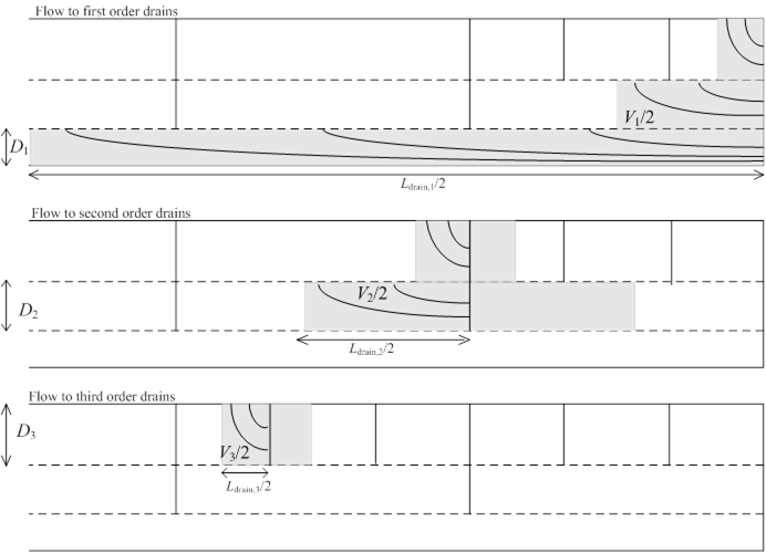
First-order drains function as field ditches and trenches, while higher-order drains act partly as third-order drains. The SWAP model computes the lumped discharge flux per drainage system from the relation between groundwater elevation and drainage resistance. Figure 4.8 illustrates the schematization of regional groundwater flow, including the occupied flow volumes for nested drain systems. The volume \(V_i\) consists of summed rectangles \(L_iD_i\) of superposed drains, where \(D_i\) is the thickness (cm) of discharge layer \(i\).
The flow volume \(V_i\) assigned to drains of order 1, 2, and 3 is related to drain distances \(L_i\) and thickness \(D_i\) of discharge layers as follows:
\[ V_1 = L_1 D_1 + L_2 D_2 + L_3 D_3 \tag{4.34}\]
\[ V_2 = L_2 D_2 + L_3 D_3 \tag{4.35}\]
\[ V_3 = L_3 D_3 \tag{4.36}\]
Rewriting Equation 4.34 to 4.36 and substituting Equation 4.32 and Equation 4.33 yields an expression which relates the proportions of the discharge layer to the discharge flow rates:
\[ L_1 D_1 : L_2 D_2 : L_3 D_3 = \left(q_\text{drain,1} L_\text{drain,1} - q_\text{drain,2} L_\text{drain,2}\right) : \left(q_\text{drain,2} L_\text{drain,2} - q_\text{drain,3} L_\text{drain,3}\right) : \left(q_\text{drain,3} L_\text{drain,3}\right) \tag{4.37}\]
Negative values for terms \(q_{\text{drain,1}} L_{\text{drain,1}} - q_{\text{drain,2}} L_{\text{drain,2}}\) indicate the absence of superposed flow systems for the corresponding drainage class. Such cases are illustrated in Figure 4.9, depicting regional groundwater flow to drains of three orders under specific conditions.
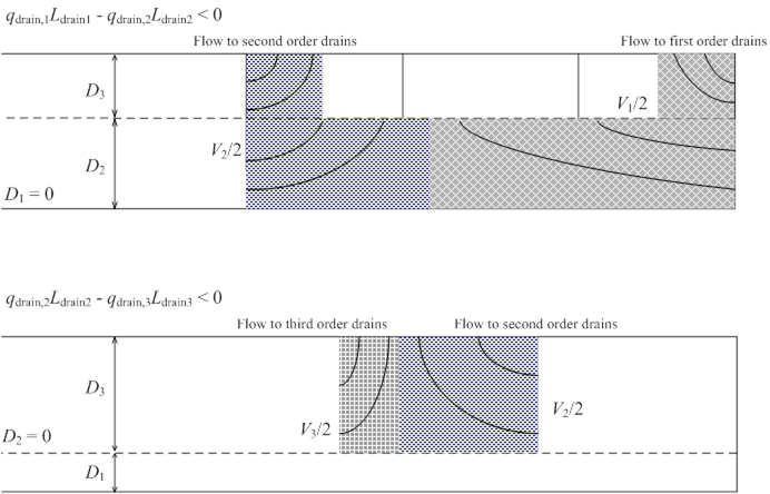
Considering soil profile stratification with respect to horizontal conductivities, Equation 4.37 is adjusted by using transmissivities instead of layer thicknesses:
\[ KD_1 : KD_2 : KD_3 = \frac{q_\text{drain,1} L_\text{drain,1} - q_\text{drain,2} L_\text{drain,2}}{L_\text{drain,1}} : \frac{q_\text{drain,2} L_\text{drain,2} - q_\text{drain,3} L_\text{drain,3}}{L_\text{drain,2}} : q_\text{drain,3} \tag{4.38}\]
Lateral drainage fluxes to a specific drainage system per nodal point are determined by the flux and the proportion of the nodal point’s transmissivity in the total transmissivity of the discharge layer.
In deep aquifers, the thickness \(D\) of a model discharge layer is constrained by:
\[ D \leq \frac{L_\text{drain}}{4} \sqrt{\frac{K_v}{K_h}} \tag{4.39}\]
where \(K_v\) and \(K_h\) represent vertical and horizontal conductivities, respectively, with weighted means used for stratified aquifers.
The top of discharge layers aligns with the average groundwater level, with solute transport to drains calculated between the simulated groundwater level and the discharge layer’s bottom. Figure 4.10 illustrates the concept, including potential overestimation of surface water load due to the defined top of the zone contributing to surface water loading.
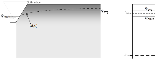
The SWAP model allows specification of the top of the zone contributing to surface water loading as a function of the average groundwater level and drainage level according to:
\[ z_\text{top} = f_\text{ztop} \phi_\text{avg} + (1 - f_\text{ztop}) \phi_\text{drain} \tag{4.40}\]
4.5 User Instructions
4.5.1 Surface Runoff
The maximum height of ponded water stored, \(h_{0,\text{threshold}}\), on the field surface is determined by the irregularities and slope of the soil surface, as well as the extent to which local field depressions are interconnected and connected to the surface water system. Typical values for \(h_{0,\text{threshold}}\) range from 0.5 to 2 cm for well-maintained agricultural fields. Since \(h_{0,\text{threshold}}\) cannot be directly measured, its value should be established through expert judgment or model calibration. This value can either be specified as a constant or set to fluctuate with time.
Surface runoff is characterized as a rapid process, thus the resistance \(\gamma\) will typically have values of less than 1 day. When the dynamics of surface runoff are of interest, the resistance \(\gamma\) (rsro) and exponent \(\beta\) (rsroexp) might need to be determined from experimental data or derived from a hydraulic model of soil surface flow.
4.5.2 Interflow
For describing the interflow process, a non-linear relation can be used. Such relation may useful for taking account for the horizontal flow in the saturated zone above drainage level may yield a non-linear relation contrary to relation based on the assumption made in the derivation of the horizontal resistance in the Ernst-equation. Another reason to introduce a non-linear relation for interflow may be the occurrence of hillslope. Sometimes it is possible to relate the parameters \(A_\text{interflow}\) and \(B_\text{interflow}\) to a specific flow concept, but most of the model user has to rely on expert judgement of model calibration.
4.5.3 Drainage
The input requirements for the simulation of a field scale drainage relation defined by a tabulated function is given in Tip 4.3.
The input requirements for the simulation of a field scale drainage relation according to Hooghoudt and Ernst is given in Tip 4.4.
The input requirements for the simulation of multi-level drainage are detailed for a basic system with fixed resistances and imposed levels in Tip 4.5, and for an extended system with surface water dependent resistances and simulated drainage levels in Tip 4.6.
Up to five different drainage levels can be specified by the user. For each level, it is possible to indicate whether drainage, infiltration, or both processes are allowed. The user must specify both the drainage and infiltration resistance. In the case of sub-irrigation, the entrance resistance (denoted as \(\gamma_\text{inf}\)) can be higher or lower than the drainage resistance (\(\gamma_\text{drain}\)), depending on local conditions. For example, a significant increase in the surface water level might lead to infiltration through a more conductive ‘bio-active’ zone, reducing the entrance resistance. Generally, with sub-irrigation, the radial resistance is higher than with drainage because the wetted section of the subsoil is smaller (the groundwater table becomes concave instead of convex). Particularly if the conductivity in the subsoil above the drainage base is greater than in the deeper subsoil, \(\gamma_\text{inf}\) will be significantly higher than \(\gamma_\text{drain}\). The model accommodates such scenarios by allowing the use of sub-irrigation resistances that differ from those used for drainage (e.g., \(\gamma_\text{inf} \approx \frac{3}{2} \gamma_\text{drain}\) as depicted in Figure 4.5).
When calibrating SWAP against measured groundwater levels, it is important to recognize that SWAP calculates a field-average groundwater level, whereas measured groundwater levels represent a specific point within the convex or concave shaped groundwater table, depending on the piezometer’s position relative to the drains. Piezometers located midway between two parallel drains will exhibit more pronounced fluctuations than the field-average level. Calibrating SWAP using these highly fluctuating groundwater levels may result in a model that inaccurately represents groundwater behavior at the field scale. To mitigate this discrepancy, it is recommended to monitor groundwater level movements using a series of piezometers arranged perpendicularly to the drain, starting from a close distance (0.5 m) to the drain, and including the drain level. This approach allows for the calculation of a shape-factor that reflects the relationship between the measured groundwater table shape and the field-average level. This shape-factor can then be used to adjust measured levels for more accurate calibration of SWAP.
The input requirements to influence the distribution of drainage fluxes with depth are given in Tip 4.7 and Tip 4.8. An implicit approach for travel times distribution (Section 4.4.1) requires specification of an anisotropy factor (cofani) for each soil layer. This factor represents the division of horizontal over vertical saturated hydraulic conductivity and will generally increase with depth. The exact location of the so-called discharge layers may be influenced by an adjustment of the upper boundary of the discharge layer (Tip 4.8 and Section 4.4.2). This adjustment requires expert judgement and it is generally not recommended to apply/adjust it without thorough knowledge of the underlying processes.